20 Multiple linear regression

Learning objectives

The learning objectives for this theme are to:

Graphically show regression problems with several predictors.
State a statistical model for linear regression with several predictors.
Compute a regression model.
Understand the difference between marginal and crude parameter estimates.
Be able to formulate hypothesis for a given question in relation to regression.

20.1 Reading material

Intro to regression
Videos on mutiple linear regression:
- Multiple Linear Regression - An Introduction
- Multiple Regression, Clearly Explained
Chapter 6.1 of Introduction to Statistics by Brockhoff

20.2 Intro to multiple linear regression

Regression models with several predictors are simply extensions of the simple linear regression with a single predictor.

A two-predictor model with $X1$ and $X2$ and a single response variable ($Y$) can be formalized as:

\[ \begin{gather} Y_i = \alpha + \beta_1 \cdot X1_i + \beta_2 \cdot X2_i + e_i \\ where \ e_i\sim \mathcal{N}(0,\sigma^2) \ and \ independent \\ for \ i=1,...,n \end{gather} \]

Where $\alpha$ refers to the level of $Y$ at $X1=X2=0$ and $\beta_1$ and $\beta_2$ are slopes in relation to $X1$ and $X2$.

Each of these three parameters consumes one degree of freedom.

The natural hypothesis is to check whether $X1$ in the presence of $X2$ has an effect on ($Y$), that is: $H0: \beta_1=0$ with the alternative $HA: \beta_1 \neq 0$ (or the other way around). This can be tested with either an F-test or a T-test (yielding the same results).

20.2.1 Marginal and Crude estimates

In a setup as described above, the investigation of the effect of $X1$ on $Y$ can be done by two approaches:

A simple regression model: $Y_i = \alpha + \beta X1_i + e_i$
A multiple regression model: $Y_i = \alpha + \beta_1 X1_i +\beta_2 X2_i + e_i$

Naturally these two approaches yield different results due to the absence/presence of the variable $X2$. From the simple regression model $\beta$ shows the crude effect of $X1$ on $Y$, whereas in the multiple regression model $\beta_1$ shows the marginal effect of $X1$ on $Y$. Sometimes comparison of these models are referred to as adjusting for $X2$ or controlling for $X2$. These models often elucidate the direct and indirect relation between predictors and responses as is seen in exercise 1.

Example 20.1

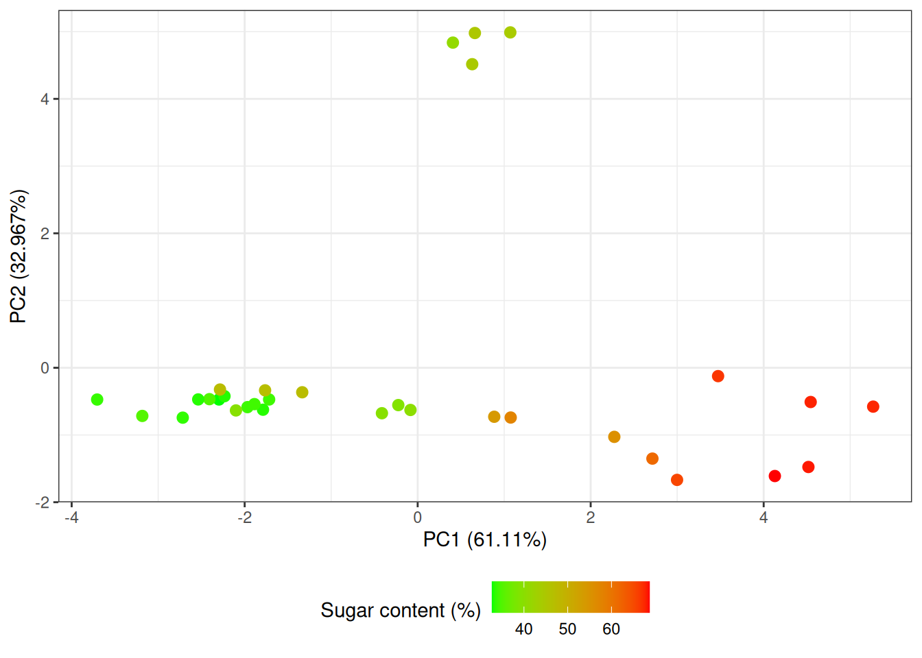
Example 20.1 - Near-infrared spectroscopy of marzipan - regression

In the following example we want to investigate if we can improve a prediction model by using scores from more than one principal component to predict the sugar content in marzipan bread (marcipanbrød).

The PCA model is exactly the same as in Example 19.1.

Code

pca <- prcomp(t(X[, -1]), center = T, scale = F)
var_exp <- summary(pca)$importance[2, ] * 100
df <- data.frame(
  pca$x,
  sugar = Y$sugar
)

ggplot(df, aes(PC1, PC2)) + 
  geom_point(size = 2.5, aes(color = sugar)) +
  scale_color_gradient(low = "green", high = "red") +
  labs(
    y = paste("PC2 (", var_exp[2], "%)", sep = ""),
    x = paste("PC1 (", var_exp[1], "%)", sep = ""),
    color = "Sugar content (%)"
  ) +
  theme_bw() +
  theme(legend.position = "bottom")

Figure 20.1: Score plot of PC1 vs PC2 on a PCA model computed on NIR spectra of marzipan samples

We now make two models:

A linear regression model on the sugar content versus the scores from PC1 (see @Example 19.1).
A linear regression model on the sugar content versus the scores from PC1 and PC2.

linreg1 <- lm(sugar ~ PC1, df)
linreg2 <- lm(sugar ~ PC1 + PC2, df)

Let us look at the summary of the two models:

summary(linreg1)


Call:
lm(formula = sugar ~ PC1, data = df)

Residuals:
    Min      1Q  Median      3Q     Max 
-7.1351 -4.3117 -0.6425  3.6072 11.6073 

Coefficients:
            Estimate Std. Error t value Pr(>|t|)    
(Intercept)  46.2531     0.8872   52.13  < 2e-16 ***
PC1           4.6208     0.3501   13.20 4.97e-14 ***
---
Signif. codes:  0 '***' 0.001 '**' 0.01 '*' 0.05 '.' 0.1 ' ' 1

Residual standard error: 5.019 on 30 degrees of freedom
Multiple R-squared:  0.8531,    Adjusted R-squared:  0.8482 
F-statistic: 174.3 on 1 and 30 DF,  p-value: 4.969e-14

summary(linreg2)


Call:
lm(formula = sugar ~ PC1 + PC2, data = df)

Residuals:
    Min      1Q  Median      3Q     Max 
-6.7699 -3.5350 -0.7164  2.7634 11.2274 

Coefficients:
            Estimate Std. Error t value Pr(>|t|)    
(Intercept)  46.2531     0.8063  57.367  < 2e-16 ***
PC1           4.6208     0.3181  14.526 7.67e-15 ***
PC2          -1.1724     0.4331  -2.707   0.0113 *  
---
Signif. codes:  0 '***' 0.001 '**' 0.01 '*' 0.05 '.' 0.1 ' ' 1

Residual standard error: 4.561 on 29 degrees of freedom
Multiple R-squared:  0.8827,    Adjusted R-squared:  0.8747 
F-statistic: 109.2 on 2 and 29 DF,  p-value: 3.178e-14

From the summary of linreg2 we see that the PC2 estimate is slightly significantly different from $0$ ($p-value = 0.01$) and does contribute to improving the model. If we think back on example Example 6.2, we learned that the second principal component had something to do with the color of the marzipan bread. In that regard it does not make a lot of sense that adding a color term (captured by the scores on PC2) into your model improve the prediction of the sugar content. However, when comparing the $R^2$ values for the model including only one component ($R^2 = 0.85$) and a model with two components ($R^2 = 0.88$) it is seen that the improvement does not practically make a difference.

One should always be careful not to build models on meaningless data. PCA is a powerful tool for exploring data, but you need to choose meaningful principal components for your analysis. This is also relevant when selecting variables for the analysis.

Maybe the wavelengths covering the visible part of the spectrum should have been left out of the analysis from the beginning as they do not contain information about the sugar content?

20.3 Videos

Multiple Linear Regression - An Introduction - Lee Rusty Waller

Multiple Regression, Clearly Explained - StatQuest

20.4 Exercises

Exercise 20.1

Exercise 20.1 - Diet and fat metabolism - regression with several variables

This exercise examines the relation between a biomarker, dietary intervention and weight in order to disentangle the effects causing elevated levels of cholesterol.

The data for this exercise is the same as for Exercise “Diet and Fat”.

In this exercise we are going to focus on predicting cholesterol from both weight and dietary intervention.

Tasks

Plot, formulate and build univariate models predicting cholesterol level from:

Dietary intervention ($Fat_Protein) - A oneway ANOVA model.
Body weight at $14$ weeks ($bw_w14) - A regression model.

State and test relevant hypothesis for these two models.
Comment on the relations between the conclusions of the two models.
Make a scatter plot of cholesterol versus weight colored or shaped according to dietary intervention.
Make a regression model for cholesterol with two predictors: i) Weight at week $14$ and ii) Dietary intervention, and test the factors.

Note: In contrast to ANOVA with one dependent variable, the order of the dependent variables makes a difference in the anova(). In order to surpass this, use the drop1(aov(),test='F') function to get results independent of order.

Tasks

What happens to the significance of the individual factors when you change the analysis as described above?
Do you think that the dietary intervention directly affects the cholesterol level, or that it is mediated through body weight?

# Multiple linear regression ```{r} #| label: mlr-setup #| echo: false #| message: false #| warning: false library(ggplot2) library(here) load(here("data", "Marzipan.RData")) ``` ::: {.callout-tip} ## Learning objectives The learning objectives for this theme are to: * Graphically show regression problems with several predictors. * State a statistical model for linear regression with several predictors. * Compute a regression model. * Understand the difference between marginal and crude parameter estimates. * Be able to formulate hypothesis for a given question in relation to regression. ::: ## Reading material * [Intro to regression ](#sec-intro-to-regression) * Videos on mutiple linear regression: * [Multiple Linear Regression - An Introduction](#sec-mlr-lee-waller) * [Multiple Regression, Clearly Explained](#sec-mlr-statquest) * Chapter 6.1 of [*Introduction to Statistics*](https://02402.compute.dtu.dk/enotes/book-IntroStatistics) by Brockhoff ## Intro to multiple linear regression Regression models with several predictors are simply extensions of the simple linear regression with a single predictor. A two-predictor model with $X1$ and $X2$ and a single response variable ($Y$) can be formalized as: $$ \begin{gather} Y_i = \alpha + \beta_1 \cdot X1_i + \beta_2 \cdot X2_i + e_i \\ where \ e_i\sim \mathcal{N}(0,\sigma^2) \ and \ independent \\ for \ i=1,...,n \end{gather} $$ Where $\alpha$ refers to the level of $Y$ at $X1=X2=0$ and $\beta_1$ and $\beta_2$ are slopes in relation to $X1$ and $X2$. Each of these three parameters consumes one degree of freedom. The natural hypothesis is to check whether $X1$ in the presence of $X2$ has an effect on ($Y$), that is: $H0: \beta_1=0$ with the alternative $HA: \beta_1 \neq 0$ (or the other way around). This can be tested with either an F-test or a T-test (yielding the same results). ### Marginal and Crude estimates In a setup as described above, the investigation of the effect of $X1$ on $Y$ can be done by two approaches: * A simple regression model: $Y_i = \alpha + \beta X1_i + e_i$ * A multiple regression model: $Y_i = \alpha + \beta_1 X1_i +\beta_2 X2_i + e_i$ Naturally these two approaches yield different results due to the absence/presence of the variable $X2$. From the simple regression model $\beta$ shows the crude effect of $X1$ on $Y$, whereas in the multiple regression model $\beta_1$ shows the marginal effect of $X1$ on $Y$. Sometimes comparison of these models are referred to as *adjusting* for $X2$ or *controlling* for $X2$. These models often elucidate the direct and indirect relation between predictors and responses as is seen in exercise 1. ::: {#exa-nir-of-marcipan-mlr}  ::: ::: {.callout-example} ### Near-infrared spectroscopy of marzipan - regression In the following example we want to investigate if we can improve a prediction model by using scores from more than one principal component to predict the sugar content in marzipan bread (marcipanbrød). The PCA model is exactly the same as in @exa-nir-marzipan-least-squares. ```{r} #| label: fig-nir-pc1-pc2 #| fig-cap: Score plot of PC1 vs PC2 on a PCA model computed on NIR spectra of marzipan samples #| code-fold: true pca <- prcomp(t(X[, -1]), center = T, scale = F) var_exp <- summary(pca)$importance[2, ] * 100 df <- data.frame( pca$x, sugar = Y$sugar ) ggplot(df, aes(PC1, PC2)) + geom_point(size = 2.5, aes(color = sugar)) + scale_color_gradient(low = "green", high = "red") + labs( y = paste("PC2 (", var_exp[2], "%)", sep = ""), x = paste("PC1 (", var_exp[1], "%)", sep = ""), color = "Sugar content (%)" ) + theme_bw() + theme(legend.position = "bottom") ``` We now make two models: * A linear regression model on the sugar content versus the scores from PC1 (see @@exa-nir-marzipan-least-squares). * A linear regression model on the sugar content versus the scores from PC1 and PC2. ```{r} linreg1 <- lm(sugar ~ PC1, df) linreg2 <- lm(sugar ~ PC1 + PC2, df) ``` Let us look at the summary of the two models: ```{r} summary(linreg1) summary(linreg2) ``` From the summary of `linreg2` we see that the PC2 estimate is slightly significantly different from $0$ ($p-value = 0.01$) and does contribute to improving the model. If we think back on example @exa-nirs-marzipan-pca, we learned that the second principal component had something to do with the color of the marzipan bread. In that regard it does not make a lot of sense that adding a color term (captured by the scores on PC2) into your model improve the prediction of the sugar content. However, when comparing the $R^2$ values for the model including only one component ($R^2 = 0.85$) and a model with two components ($R^2 = 0.88$) it is seen that the improvement does not practically make a difference. One should always be careful not to build models on meaningless data. PCA is a powerful tool for exploring data, but you need to choose meaningful principal components for your analysis. This is also relevant when selecting variables for the analysis. Maybe the wavelengths covering the visible part of the spectrum should have been left out of the analysis from the beginning as they do not contain information about the sugar content? :::  ## Videos #### Multiple Linear Regression - An Introduction - *Lee Rusty Waller* {#sec-mlr-lee-waller} {{< video https://www.youtube.com/watch?v=G4ZlC9zKfII >}} #### Multiple Regression, Clearly Explained - *StatQuest* {#sec-mlr-statquest} {{< video https://www.youtube.com/watch?v=EkAQAi3a4js >}} ## Exercises ::: {#ex-diet-mlr}  ::: ::: {.callout-exercise} ### Diet and fat metabolism - regression with several variables This exercise examines the relation between a biomarker, dietary intervention and weight in order to disentangle the effects causing elevated levels of cholesterol. The data for this exercise is the same as for Exercise "Diet and Fat". In this exercise we are going to focus on predicting cholesterol from both weight and dietary intervention. ::: {.callout-task} 1. Plot, formulate and build univariate models predicting cholesterol level from: a. Dietary intervention (`$Fat_Protein`) - A oneway ANOVA model. b. Body weight at $14$ weeks (`$bw_w14`) - A regression model. 2. State and test relevant hypothesis for these two models. 3. Comment on the relations between the conclusions of the two models. 4. Make a scatter plot of cholesterol versus weight colored or shaped according to dietary intervention. 5. Make a regression model for cholesterol with two predictors: i) Weight at week $14$ and ii) Dietary intervention, and test the factors. ::: Note: In contrast to ANOVA with one dependent variable, the order of the dependent variables makes a difference in the `anova()`. In order to surpass this, use the `drop1(aov(),test='F')` function to get results independent of order. ::: {.callout-task} 6. What happens to the significance of the individual factors when you change the analysis as described above? 7. Do you think that the dietary intervention *directly* affects the cholesterol level, or that it is mediated through body weight? ::: :::