# Load data
load("Marzipan.RData")19 Least squares
Learning objectives
The learning objectives for this theme is to understand the mathematical formulation of least squares problems. That is:
- Be able to formulate an objective given a model. The objective function represents what we are trying to minimize or optimize.
- Understand how the first derivative of the objective is interesting. Taking derivatives helps us find the minimum of the objective function and optimal parameter values.
- For the most simple examples, with one and two parameters, be able to state the analytical solution that minimizes the objective. Understanding these basic cases builds intuition for more complex scenarios.
- Based on data, give least squares central estimates for parameters. This involves applying the method to real data to estimate model parameters.
- Know that this is a very generic framework, which is conducted “under the shelf” by computer algorithms. The same principles apply across many statistical methods.
- Relate least squares to PCA, ANOVA, linear regression and correlation analysis. Understanding how these common statistical methods are connected through least squares optimization.
19.1 Reading material
- Least squares - in short
- Videos on least squares and linear regression
- Chapter 5.1 and 5.2 of Introduction to Statistics by Brockhoff
19.2 Least squares - in short
A model (ANOVA, linear regression, PCA,…) can be seen as a representation of the observed data, such that:
\[ Observed = Systematic + Residuals \]
Here the aim is to choose some parameters for the systematic part, which makes the residuals small. Specifically small often refers to a small sum of squares. Brockhoff describes the case for linear regression, so here we will mention ANOVA problems and PCA.
19.2.1 ANOVA - least Squares
The formula for an additive ANOVA model with two factors is listed below:
\[ \begin{gather} X_{i} = \alpha(A_i) + \beta(B_i) + e_{i} \\ where \ e_{i}\sim \mathcal{N}(0,\sigma^2) \ and \ independent \\ for \ i=1,...,n \end{gather} \]
In this case the aim is to estimate some numbers for the parameters (\(\alpha(1),..,\alpha(k_A)\), and \(\beta(1),..,\beta(k_B)\)) - \(k_A + k_B\) in total - such that \(\sum{e_i^2}\) is as small as possible. For what is called balanced studies, it turns out that using the group means within each factor, as estimates for \(\alpha()\) and \(\beta()\), gives the least \(\sum{e_i^2}\) (sum of squared errors). The proof for this is found by calculating \(\sum{e_i^2}\):
\[ L = \sum_{i=1}^n{e_i^2} =\sum_{i=1}^n{(X_{i} - \alpha(A_i) + \beta(B_i))^2} \]
Differentiation of this and setting it to zero:
\[ \frac{\delta L}{\delta \alpha,\delta \beta} = .... = 0 \]
Followed by isolation of the parameters, it is possible to derive the estimates. These are called the Least Squares estimates.
The math is very similar to regression. It is however, beyond the curriculum to be able to do it for ANOVA and PCA problems.
19.2.2 Principal Component Analysis - least squares
In PCA the multivariate dataset (\(\mathbf{X}\)) is parameterized by scores (\(\mathbf{T}\)) and loadings (\(\mathbf{P}\)):
\[ \mathbf{X} = \mathbf{T}\mathbf{P}^T + \mathbf{E} \tag{1} \]
Contrary to the univariate cases mentioned above, the data and parameters are here matrices, however, the aim is still to find some scores and loadings that minimizes \(\mathbf{E}\) in a least squares sense: \(\sum{\mathbf{E}_{ij}^2}\), where \(i\) refers to the sample \(i\) and \(j\) refers to variable \(j\). I.e. \(\mathbf{E}_{3,4}\) is the residual for sample \(3\) variable \(4\).
Example 19.1 - Near-infrared spectroscopy of marzipan - least squares
The following example illustrates how we can use scores from a principal component analysis to predict the sugar content in marzipan bread (marcipanbrød).
First we import the data. It is saved as an RData-file, so that is easy.
Then we can plot the data.
# Plot data colored according to sugar content
ggplot(Xm, aes(wavelength, value, color = sugar)) +
  geom_line() +
  scale_color_gradient(low = "green", high = "red") +
  labs(
    y = "Absorbance",
    x = "Wavelength (nm)",
    title = "NIR spectrum of marzipan",
    color = "Sugar content (%)"
  ) +
  theme_bw() +
  theme(
    legend.position = "bottom",
    plot.title = element_text(hjust = 0.5, face = "bold")
    )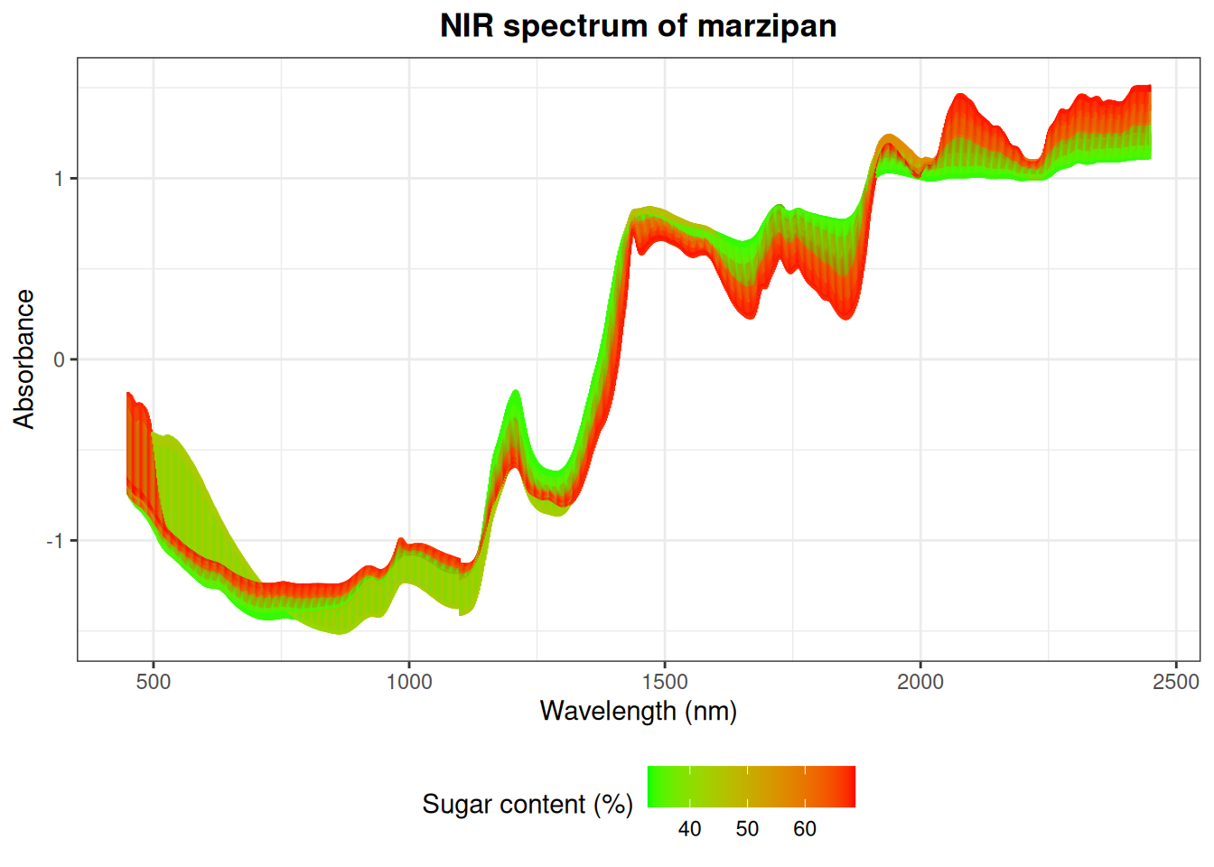
In this example we want to make a model which can predict the sugar content from a spectrum.
We now make a PCA on the data and plot PC1 vs sugar content.
# Transposing the data and removing the "wavelength" column
Xt = t(X[, -1])

# Compute a PCA model on meant centered Xt
pca <- prcomp(Xt, center = T, scale = F)

# Extract the scores from the PCA model and the sugar content from data
df <- data.frame(
  scores = pca$x,
  sugar = Y$sugar
)

# Extract the variance explained (%) for PC1
var_exp_pc1 <- summary(pca)$importance[2, 1] * 100

# Plot PC1 scores vs sugar content. Color points according to sugar content
ggplot(df, aes(scores.PC1, sugar)) +
  geom_point(size = 2.5, aes(color = sugar)) +
  scale_color_gradient(low = "green", high = "red") +
  geom_smooth(method = "lm", se = F) + # Show regression line
  labs(
    y = "Sugar content (%)",
    x = paste("PC1 (", var_exp_pc1, "%)", sep = ""), # Add var.exp% as label
    color = "Sugar content (%)"
  ) +
  theme_bw() +
  theme(legend.position = "bottom")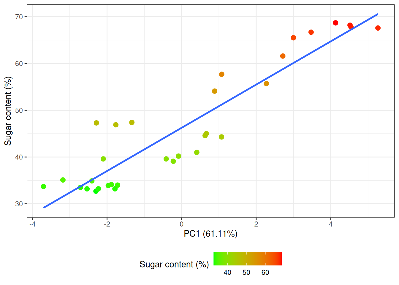
There is indeed a linear relation between the scores on PC1 and the sugar content in the marzipan breads. Let us make a linear regression model using the least squares approach with sugar content as dependent variable and the scores from PC1 as predictors:
linreg = lm(sugar ~ scores.PC1, df)From which we can extract the intercept, slope and \(R^2\):
summary(linreg)$r.squared[1] 0.8531228linreg$coefficients(Intercept) scores.PC1
46.253124 4.620843 Our model of sugar content (\(Y\)) can be written as:
\[ Y = 4.6 \cdot PC1_{scores} + 46.3 \]
This model is explaining \(85\%\) of the variance of the response variable (sugar content).