Introduce the predominant distribution within biological data; The normal distribution.
Be able to characterize the distribution by a set of parameters, and be able to calculate the precision of these parameters (give confidence intervals) based on data.
Know which graphics that are useful for visualizing normally distributed data (histogram, boxplot, qq-plot), and be able to use this to judge whether normality is fulfilled.
For a given distribution to be able to calculate the probability of a given observation.
Especially 2.1 to 2.4 (you can skip 2.2 on discrete distributions, which is the subject of week 4) and 3.1 - 3.1.6.
8.2 The normal distribution - in short
If \(X\) is normaly distributed with mean \(\mu\) and variance \(\sigma^2\), then the probability density function for a given draw from that distribution \(x\) is given by
Further, the cumulative density function can be found by integration of this formula \[
P(X \leq x) = \frac{1}{{\sigma \sqrt {2\pi } }} \int_{-\inf}^x e^{{{ - \left( {x - \mu } \right)^2 } {2\sigma ^2 }}} \, dx
\]
The short notation for this distribution is
\[
X \sim \mathcal{N}(\mu,\sigma^2)
\]
8.2.1 Estimation of \(\mu\) and \(\sigma\)
More often than not, the distribution is unknown. That is the values of \(\mu\) and \(\sigma\) are unknown and must then be estimated from data.
\(\mu\) characterizes the center of the distribution, and is naturally estimated by the mean-value of the data-points (\(\bar{X}\)). \(\sigma\) reflects the spread around the mean, and is in a similar fashion estimated by the standard deviation (\(\hat{\sigma}\) or \(s\)).
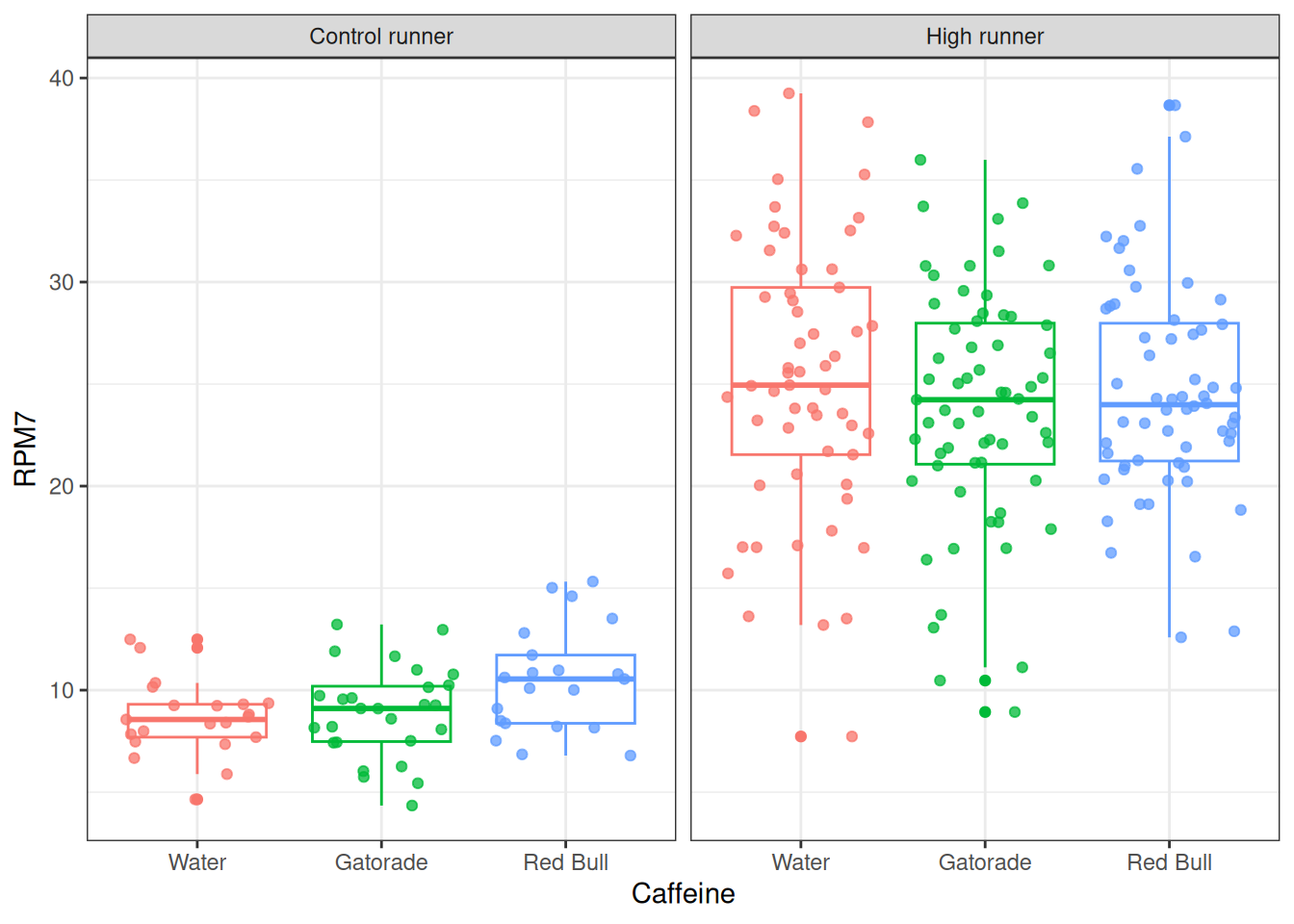
Caffeine is a central neurvous system stimulant, which can have several positive- and negative effects. In this study, the level of activity is up for examination, and for this purpose a model-system; the runing activity of mice in a wheel reflected as the number of rounds pr minutes recorded over 7 minutes. Here a total of 249 mice from two species; one breed to be high in running performance, and one control, where given either Water, Gatorade or Red Bull followed by measuring their voluentary wheel run activiy. Of interest is the average actvity within each mouse type and for each caffeine type and how large the spread is.
The data is listed in a table with 249 rows (here, the first five samples are shown):
head(X)
       MouseType gender Caffeine    RPM7
1 Control runner   Male Red Bull 10.5461
2    High runner Female Gatorade 24.2718
3    High runner Female Gatorade 19.7215
4 Control runner   Male Red Bull 13.5099
5 Control runner   Male Red Bull 15.3210
6    High runner   Male Gatorade 30.7953
To get the experimental design, the table() function nicely summarize the numbers within each group:
Figure 8.1: Box n’ jitter plot of the RPM7 variable as a function of treatment.
As an example, the mean and standard deviation is calculated for females of the unselected breed given water. The example is given using both base R and Tidyverse.
And then the extracted information can be fed into the mean() and sd() functions.
mean(extracted_x)
[1] 8.649382
sd(extracted_x)
[1] 2.07804
In Tidyverse the filter-function is used to filter by the MouseType, gender, and Caffeine levels of interest. Afterwards, the mean and standard deviation are computed using summarise.
A more efficient way of doing this would be to calculate the mean and standard deviation of each combination and display them in a table. The example below is given using both base R and Tidyverse.
In base R aggregate() can be used to calculate a function over a group.
# Compute number of observations, mean and sd across groupsn <-aggregate(X$RPM7, by =list(X$MouseType, X$gender, X$Caffeine), length)m <-aggregate(X$RPM7, by =list(X$MouseType, X$gender, X$Caffeine), mean)s <-aggregate(X$RPM7, by =list(X$MouseType, X$gender, X$Caffeine), sd)# Combine and set column namesstat_table <-cbind(n, m$x, s$x)colnames(stat_table) <-c("MouseType","Gender","Caffeine","N","mean","sd")# Print as nice markdown tablekable(stat_table, digits =2)
MouseType
Gender
Caffeine
N
mean
sd
Control runner
Male
Water
10
8.55
1.59
High runner
Male
Water
29
26.03
6.35
Control runner
Female
Water
11
8.65
2.08
High runner
Female
Water
28
24.59
7.25
Control runner
Male
Gatorade
14
8.55
2.09
High runner
Male
Gatorade
31
25.04
5.52
Control runner
Female
Gatorade
13
9.31
2.42
High runner
Female
Gatorade
32
22.65
5.86
Control runner
Male
Red Bull
12
10.73
2.95
High runner
Male
Red Bull
29
24.81
3.65
Control runner
Female
Red Bull
9
10.18
2.14
High runner
Female
Red Bull
31
24.50
6.50
In Tidyverse, the group_by()-function is used to group the observations by everything but the column RPM7 (so that will be type, gender and caffeine). Then, the number of observations, mean and standard devations are calculated across groups, giving the information for each group in one go.
X |>group_by(across(-RPM7)) |>summarise(N =n(),mean =mean(RPM7),sd =sd(RPM7) ) |>kable(digits =2) # Output pretty table in markdown
`summarise()` has grouped output by 'MouseType', 'gender'. You can override
using the `.groups` argument.
MouseType
gender
Caffeine
N
mean
sd
Control runner
Male
Water
10
8.55
1.59
Control runner
Male
Gatorade
14
8.55
2.09
Control runner
Male
Red Bull
12
10.73
2.95
Control runner
Female
Water
11
8.65
2.08
Control runner
Female
Gatorade
13
9.31
2.42
Control runner
Female
Red Bull
9
10.18
2.14
High runner
Male
Water
29
26.03
6.35
High runner
Male
Gatorade
31
25.04
5.52
High runner
Male
Red Bull
29
24.81
3.65
High runner
Female
Water
28
24.59
7.25
High runner
Female
Gatorade
32
22.65
5.86
High runner
Female
Red Bull
31
24.50
6.50
Example 8.2
Example 8.2 - Effect of caffeine on activity - probability
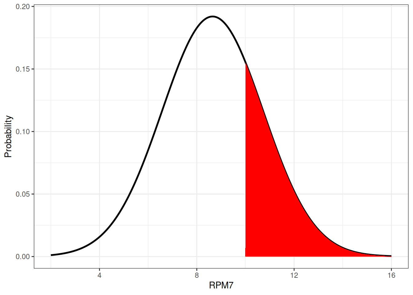
Example Example 8.1 estimates the activity distribution of mice based on experimental data. Under the assumption that these metrics, the mean and the standard deviation, perfectly describe the distribution of the data, and further that this distribution is the normal distribution, we wish to calculate the probability of a given female mice, from normal breed, assigned water to perform higher than 10 RPM7.
where \(X\) is assummed normally distributed with mean \(\mu\) and standard deviation \(\sigma\).
That is: \(X \sim \mathcal{N} (\mu,\sigma^2)\). \
A small illustration below (figure 8.2) shows the area of interest.
# Create normal distributed data using estimated mean and sddf <-data.frame(x =seq(2, 16, 0.01)) |>mutate(y =dnorm(x, mean(extracted_x), sd(extracted_x))) # Plot normal curve ggplot(df, aes(x, y)) +geom_line(linewidth =1) +geom_area(data =subset(df, x >=10), fill ="red") +labs(x ="RPM7",y ="Probability" ) +theme_bw()
Figure 8.2: Normal density function fitted to the selected mouse population. The red area is the density for RPM7 >= 10.
The size of the red area is simply calculated via the pnorm() function.
1-pnorm(10, mean(extracted_x), sd(extracted_x))
[1] 0.2578628
\[
P(X \geq 10) \approx 0.26
\]
The probability of a single female mice, from normal breed, administered with water to perform higher than \(10 RPM7\) is hence \(0.26\).
8.2.2 Confidence interval for \(\mu\)
The confidence interval for the center of a normal distribution (\(\mu\)) is calculated as follows:
where \(t_{1-\alpha/2,df}\) is a fractile, a number, which determines the coverage. Here, \(\alpha\) is the left ot part. I.e. if a \(90 \%\) confidence interval is wanted, the left out part is \(\alpha = 0.10\). \(n\) is the number of samples on which the mean (\(\bar{X}\)) is estimated, and \(df\) is the degrees of freedom, which refers to how well the standard deviation is estimated.
For instance, if one needs a \(95 \%\) confidence interval (\(\alpha = 0.05\)) based on a sample of \(20\) observations \(t_{1-\alpha/2,df} = t_{0.975,20-1} = 2.093\).
It is further noticed that the interval is symmetric around the mean, and that the more samples (\(n\)) the lower the spread as the standard deviation is divided by \(\sqrt{n}\).
Example 8.3
Example 8.3 - Effect of caffeine on activity - confidence intervals
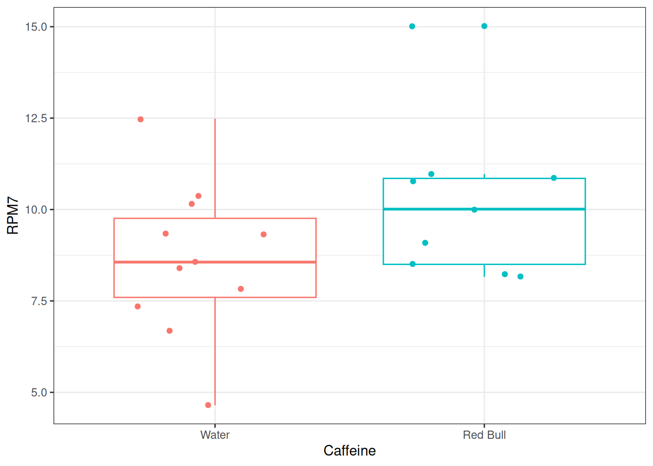
In example Example 8.1 concerning the relation between caffeine and voluntary activity of mice, the running activity of mice in a wheel is recorded. In this example we wish to estimate the mean activity of the two groups with either water- or Red bull as caffeine source in control runner female mice, and give a confidence interval for these means.
First, the data is subset to only include the two groups of interest.
After subsetting the data to only include these two groups a plot of the raw data looks like the following, and consists of \(n = n_1 + n_2 = 11+ 9 = 20\) samples (figure 8.3).
Figure 8.3: Box n’ jitter plot of the mouse data subset.
The mean and standard deviation for the two groups can be calculated using summarise() via Tidyverse or aggregate() in base R (see Example 8.1 for an example on aggregate).
x_subset |>group_by(Caffeine) |>summarise(N =n(),mean =mean(RPM7),sd =sd(RPM7) ) |>kable(digits =2) # For pretty tables in markdown
With a total of \(df_1 = n_1 - 1 = 10\) degress of freedom the t-fractileat level \(95 \%\) is \(t_{0.975,10} = 2.23\) why the confidence interval for the water treated group is:
n <-11# Number of obs in water groupt_frac <-qt(1-0.05/2, n -1) # T-values <-sd(x_subset[x_subset$Caffeine =="Water", "RPM7"])m <-mean(x_subset[x_subset$Caffeine =="Water", "RPM7"])ci_lower <- m - t_frac * s /sqrt(n)ci_upper <- m + t_frac * s /sqrt(n)cat("95% confidence interval for water group:\n", c(ci_lower, ci_upper))
95% confidence interval for water group:
 7.253336 10.04543
    One Sample t-test

data:  x_subset[x_subset$Caffeine == "Water", "RPM7"]
t = 13.805, df = 10, p-value = 7.744e-08
alternative hypothesis: true mean is not equal to 0
95 percent confidence interval:
  7.253336 10.045428
sample estimates:
mean of x
 8.649382
8.3 Videos
8.3.1 The Normal Distribution - CrashCourse
8.3.2 An Introduction to the Normal Distribution - jbstatistics
8.3.3 The Normal Distribution, Clearly Explained - StatQuest
8.3.4 Confidence Intervals - CrashCourse
8.4 Exercises
Exercise 8.1
Exercise 8.1 - Normal Distribution
Serum cholestorol level is a biomarker of health in relation to a range of life-style related diseases. A population of adults have mean values of \(178 mg/100mL\) and \(207 mg/100mL\), standard deviations of \(31 mg/100mL\) and \(37 mg/100mL\) in males and females respectively.
Tasks
Draw curves (by hand - with pen on paper!) and plug in the parameters for these distributions.
What percentage are below \(150, 178\) and \(200 mg/100 mL\) respectively (for males and females separately)?
What percentage are above \(140 mg/100 mL\)
A level above \(240 mg/100 mL\) is considered high risk, whereas the range between \(200\) and \(239 mg/100 mL\) is considered borderline high risk.
Tasks
How big a proportion is considered at high risk (for males and females seperately)?
How big a proportion is considered borderline high risk (for males and females seperately)?
Now assume that the above metrics describing the distribution (mean and standard deviation) is estimated based on samples of \(30\) males and \(30\) females. What it the changes to the calculations above?
A population consists of \(40\%\) males and \(60\%\) females.
Tasks
What is the propability that a random person from that population have a serum cholesterol level higher than \(240 mg/100mL\).
Use that the mean and variance of a sum of two populations is the sum of the means and variance respectively. That is; Let \(X\) and \(Y\) be two indepedent random variables with mean \(\mu_X\) and \(\mu_y\) and variance \(\sigma^2_X\) and \(\sigma^2_Y\) respectively. And let:
\[
Z = c_1X+ c_2Y
\]
Then the mean and variance of \(Z\) is: \[
\mu_Z = c_1\mu_X + c_2\mu_Y
\]\[
\sigma^2_Z = c_1\sigma^2_X + c_2\sigma^2_Y
\]
Tasks
What is the population mean and standard deviation of a population made up of \(40\%\) males and \(60\%\) females?
Use this mean and standard deviation to calculate the probability of a random person from that population having a serum cholesterol level higher than \(240 mg/100mL\). How is that different from question 7? and why so?
Exercise 8.2
Exercise 8.2 - Transformations and the normal distribution
The normal distribution (also known as the Gaussian distribution) are central in biology as such, and in data analysis especially.
Tasks
Why do we (sometimes) transform data before making statistical analysis?
Make a histogram plot and a qqplot (use qqnorm() and qqline() functions) on the variable Ethyl.pyruvate from the “Wine” data set. Are the data normal distributed?
Try to Log transform the variable Ethyl.pyruvate. Make a new histogram plot and a corresponding qqplot. Compare with question 1.
Use the command par(mfrow = c(1,2)) (in front of your plotting commands) to get the plots side by side which makes it easier to compare the results.
Add a suitable title on both plots using the argument main="a very nice title".
Does it seem possible to get all samples to match the same distribution?
Do the same for the variable Benxyl.alcohol.
Does the log transformation work? What is the problem?
Try the square root transformation.
Exercise 8.3
Exercise 8.3 - WHO height and weight - standard normal distribution
Height and weight are important measures of growth during childhood. However, the largest factor impacting these measures are naturally the age of the child. In order to be able to compare children with slightly different ages such data are transformed using so-called growth curves. These are provided by the WHO and are constructed to represent the world wide distribution at specific ages for boys and girl. In this exercise you are supposed to take height and weight measures from African children living under different circumstances, transform them using WHO numbers for the world wide distribution, and further look for explanatory variables causing differences in growth.
Tasks
Start by importing the GrowthData.xlsx dataset into R. Check that all the info from the excel file was imported correctly using the commands dim() and head(). You can ’chop’ the dataframe in R to isolate the variables of importance (length, sex, age etc.).
Using the following graphs (figure 8.4), find the mean and standard deviation for boys and girls at age 15 months.
(a) Z-scores for the length-to-age ratio for girls
(b) Z-scores for the length-to-age ratio for boys.
Figure 8.4: Z-scores for the length-to-age ratio for girls and boys aged 0 to 2 years. Source: WHO. Click on the images to enlargen them.
Tasks
Based on the dataset imported, calculate mean and standard deviation for the girls and the boys, how does it relate to the data from WHO?
You can use the command X <- X[complete.cases(X),] to remove the empty rows in the dataframe X, or google how to compute descriptive statistics in the case of missing values.
Tasks
What is the Z-value? How can you use it to relate the dataset to the WHO data?
Calculate the Z-scores for all the boys and girls.
This can be done by creating a new vector inserting the length-vector from the previous dataframe to the equation for Z-score.
Tasks
What does it mean that a child is above or below 0 in Z-score? How many children has a Z-score below -2 and -3?
How many children are longer/taller than the world average?
Investigate whether some of the other variables (source of water primary_watersource or treatment of water water_treatment_type) impact the length at 15 months. Use ggplot() to do the plotting, and then use ggplot(...) + facet_wrap(~SEX) to split the plot in two corresponding to the variable SEX. Are the trends similar for the two sexes?
Source Code
# The normal distribution```{r}#| label: normal dist setup#| echo: false#| message: false#| warning: falselibrary(kableExtra)library(here)library(ggplot2)library(dplyr)load(here("data", "MouseWheelCaffeine.RData"))```::: {.callout-tip}## Learning objectives* Introduce the predominant distribution within biological data; The normal distribution. * Be able to characterize the distribution by a set of parameters, and be able to calculate the precision of these parameters (give confidence intervals) based on data. * Know which graphics that are useful for visualizing normally distributed data (histogram, boxplot, qq-plot), and be able to use this to judge whether normality is fulfilled. * For a given distribution to be able to calculate the probability of a given observation.:::## Reading material* [The normal distribution - in short](#sec-intro-to-normal)* Videos giving short condensed introduction to the normal distribution: * [The Normal Distribution](#sec-the-normal-distribution) * [An Introduction to the Normal Distribution](#sec-intro-to-the-normal-distribution) * [The Normal Distribution, Clearly Explained](#sec-the-normal-distribution-clearly-explained)* Video on confidence intervals: * [Confidence intervals](#sec-confidence-intervals)* Chapter 2 and 3 of [*Introduction to Statistics*](https://02402.compute.dtu.dk/enotes/book-IntroStatistics) by Brockhoff * Especially 2.1 to 2.4 (you can skip 2.2 on discrete distributions, which is the subject of week 4) and 3.1 - 3.1.6.## The normal distribution - in short {#sec-intro-to-normal}If $X$ is normaly distributed with mean $\mu$ and variance $\sigma^2$, then the probability density function for a given draw from that distribution $x$ is given by $$P(x) = \frac{1}{{\sigma \sqrt {2\pi } }}e^{{{ - \left( {x - \mu } \right)^2 } {2\sigma ^2 }}}$$Further, the cumulative density function can be found by integration of this formula$$P(X \leq x) = \frac{1}{{\sigma \sqrt {2\pi } }} \int_{-\inf}^x e^{{{ - \left( {x - \mu } \right)^2 } {2\sigma ^2 }}} \, dx$$The short notation for this distribution is$$X \sim \mathcal{N}(\mu,\sigma^2)$$### Estimation of $\mu$ and $\sigma$ {#sec-estimation-of-parameters}More often than not, the distribution is unknown. That is the values of $\mu$ and $\sigma$ are unknown and must then be estimated from data.$\mu$ characterizes the center of the distribution, and is naturally estimated by the mean-value of the data-points ($\bar{X}$). $\sigma$ reflects the spread around the mean, and is in a similar fashion estimated by the standard deviation ($\hat{\sigma}$ or $s$). $$\hat{\mu} = \bar{X} = \sum_{i = 1}^n X_i / n = (X_1 + X_2 + X_3 + \ldots + X_n) / n$$$$\hat{\sigma}^2 = s^2 = \sum_{i = 1}^n (X_i - \bar{X})^2 / (n-1) = ((X_1 - \bar{X})^2 + (X_2 - \bar{X})^2 + (X_3 - \bar{X})^2 + \ldots + (X_n - \bar{X})^2 ) / (n-1)$$::: {#exa-effect-of-caffeine}<!-- Cross-ref anchor -->:::::: {.callout-example}### Effect of caffeine on activityCaffeine is a central neurvous system stimulant, which can have several positive- and negative effects. In this study, the level of activity is up for examination, and for this purpose a model-system; the runing activity of mice in a wheel reflected as the number of rounds pr minutes recorded over 7 minutes. Here a total of 249 mice from two species; one breed to be high in running performance, and one control, where given either Water, Gatorade or Red Bull followed by measuring their voluentary wheel run activiy. Of interest is the average actvity within each mouse type and for each caffeine type and how large the spread is.The data is listed in a table with 249 rows (here, the first five samples are shown):```{r}head(X)```To get the experimental design, the table() function nicely summarize the numbers within each group:```{r}table(X$gender:X$MouseType, X$Caffeine)```Before doing anything else, the data is plotted to visualize the response as function of the design (@fig-caffeine-vs-rpm).```{r}#| label: fig-caffeine-vs-rpm#| fig-cap: Box n' jitter plot of the RPM7 variable as a function of treatment. ggplot(X, aes(Caffeine, RPM7, color = Caffeine)) +geom_boxplot() +geom_jitter(alpha = .75) +# Alpha controls opacityfacet_wrap(~MouseType) +theme_bw() +theme(legend.position ="none") # Remove the legend```As an example, the mean and standard deviation is calculated for females of the unselected breed given water. The example is given using both base R and Tidyverse.::: {.panel-tabset}#### Using base RFirst, the information is extracted from the dataset:```{r}extracted_x <- X[ X$MouseType =="Control runner"& X$gender =="Female"& X$Caffeine =="Water", # Rows"RPM7"] # Column```And then the extracted information can be fed into the `mean()` and `sd()` functions.```{r}mean(extracted_x)sd(extracted_x)```#### Using TidyverseIn Tidyverse the `filter`-function is used to filter by the `MouseType`, `gender`, and `Caffeine` levels of interest. Afterwards, the mean and standard deviation are computed using `summarise`. ```{r}X |>filter( MouseType =="Control runner", gender =="Female", Caffeine =="Water" ) |>summarise(mean =mean(RPM7),sd =sd(RPM7) )```::: <!-- End tabset -->Both methods output a mean and standard deviation of $$\bar{x} = \sum_{i=1}^{n} \frac{x_i}{n} \approx 8.6$$$$\hat{\sigma} = \sum_{i=1}^{n} \frac{(x_i - \bar{x})}{n - 1} \approx 2.1$$for the particular group of interest.A more efficient way of doing this would be to calculate the mean and standard deviation of each combination and display them in a table. The example below is given using both base R and Tidyverse.::: {.panel-tabset}#### Using base RIn base R `aggregate()` can be used to calculate a function over a group. ```{r}# Compute number of observations, mean and sd across groupsn <-aggregate(X$RPM7, by =list(X$MouseType, X$gender, X$Caffeine), length)m <-aggregate(X$RPM7, by =list(X$MouseType, X$gender, X$Caffeine), mean)s <-aggregate(X$RPM7, by =list(X$MouseType, X$gender, X$Caffeine), sd)# Combine and set column namesstat_table <-cbind(n, m$x, s$x)colnames(stat_table) <-c("MouseType","Gender","Caffeine","N","mean","sd")# Print as nice markdown tablekable(stat_table, digits =2)```#### Using TidyverseIn Tidyverse, the `group_by()`-function is used to group the observations by everything but the column `RPM7` (so that will be type, gender and caffeine). Then, the number of observations, mean and standard devations are calculated across groups, giving the information for each group in one go.```{r}X |>group_by(across(-RPM7)) |>summarise(N =n(),mean =mean(RPM7),sd =sd(RPM7) ) |>kable(digits =2) # Output pretty table in markdown```::: <!-- End tabset -->:::<!-- End example callout -->::: {#exa-effect-of-caffeine-probability}<!-- Cross-ref anchor -->:::::: {.callout-example}### Effect of caffeine on activity - probabilityExample @exa-effect-of-caffeine estimates the activity distribution of mice based on experimental data. Under the assumption that these metrics, the mean and the standard deviation, perfectly describe the distribution of the data, and further that this distribution is the normal distribution, we wish to calculate the probability of a given female mice, from normal breed, assigned water to perform *higher than 10 RPM7*.That is: \begin{align*}P(X \geq 10) &= \frac{1}{\sqrt{2\pi\sigma^2}}\int_{10}^{\infty} e^{-\frac{(z - \mu)^2}{2\sigma}} dz \\&= 1 - P(X < 10) \\%X &= X \\%X &= X&= 1 - \frac{1}{\sqrt{2\pi\sigma^2}}\int_{-\infty}^{10} e^{-\frac{(z - \mu)^2}{2\sigma}} dz \\%N(x) = \frac{1}{\sqrt{2\pi}}\int_{-\infty}^{x} e^{-\frac{1}{2}z^2} dz\end{align*}where $X$ is assummed normally distributed with mean $\mu$ and standard deviation $\sigma$. That is: $X \sim \mathcal{N} (\mu,\sigma^2)$. \\A small illustration below (@fig-normal-dist-rpm7) shows the area of interest.```{r}#| label: fig-normal-dist-rpm7#| fig-cap: Normal density function fitted to the selected mouse population. The red area is the density for RPM7 >= 10. # Create normal distributed data using estimated mean and sddf <-data.frame(x =seq(2, 16, 0.01)) |>mutate(y =dnorm(x, mean(extracted_x), sd(extracted_x))) # Plot normal curve ggplot(df, aes(x, y)) +geom_line(linewidth =1) +geom_area(data =subset(df, x >=10), fill ="red") +labs(x ="RPM7",y ="Probability" ) +theme_bw()```The size of the red area is simply calculated via the `pnorm()` function.```{r}1-pnorm(10, mean(extracted_x), sd(extracted_x))```$$P(X \geq 10) \approx 0.26$$The probability of a single female mice, from normal breed, administered with water to perform higher than $10 RPM7$ is hence $0.26$. :::<!-- End example callout -->### Confidence interval for $\mu$The confidence interval for the center of a normal distribution ($\mu$) is calculated as follows: $$CI_{\mu,1-\alpha}: \hat{\mu} \pm t_{1-\alpha/2,df} \cdot \hat{\sigma} / \sqrt(n)$$$$\bar{X} \pm t_{1-\alpha/2,df} \cdot s / \sqrt(n) $$where $t_{1-\alpha/2,df}$ is a fractile, a number, which determines the coverage. Here, $\alpha$ is the left ot part. I.e. if a $90 \%$ confidence interval is wanted, the left out part is $\alpha = 0.10$. $n$ is the number of samples on which the mean ($\bar{X}$) is estimated, and $df$ is the degrees of freedom, which refers to how well the standard deviation is estimated. For instance, if one needs a $95 \%$ confidence interval ($\alpha = 0.05$) based on a sample of $20$ observations $t_{1-\alpha/2,df} = t_{0.975,20-1} = 2.093$.It is further noticed that the interval is symmetric around the mean, and that the more samples ($n$) the lower the spread as the standard deviation is divided by $\sqrt{n}$. ::: {#exa-effect-of-caffeine-conf-int}<!-- Cross-ref anchor -->:::::: {.callout-example}### Effect of caffeine on activity - confidence intervalsIn example @exa-effect-of-caffeine concerning the relation between caffeine and voluntary activity of mice, the running activity of mice in a wheel is recorded. In this example we wish to estimate the mean activity of the two groups with either water- or Red bull as caffeine source in control runner female mice, and give a confidence interval for these means. First, the data is subset to only include the two groups of interest. ```{r}x_subset <- X |>filter( MouseType =="Control runner", gender =="Female", Caffeine %in%c("Red Bull", "Water") )```After subsetting the data to only include these two groups a plot of the raw data looks like the following, and consists of $n = n_1 + n_2 = 11+ 9 = 20$ samples (@fig-mouse-subset).```{r}#| label: fig-mouse-subset#| fig-cap: Box n' jitter plot of the mouse data subset. ggplot(x_subset, aes(Caffeine, RPM7, color = Caffeine)) +geom_boxplot() +geom_jitter() +theme_bw() +theme(legend.position ="none") # Remove legend```The mean and standard deviation for the two groups can be calculated using `summarise()` via Tidyverse or `aggregate()` in base R (see @exa-effect-of-caffeine for an example on `aggregate`).```{r}x_subset |>group_by(Caffeine) |>summarise(N =n(),mean =mean(RPM7),sd =sd(RPM7) ) |>kable(digits =2) # For pretty tables in markdown```The confidence interval is calculated as follows: \begin{align}CI_{\mu}: & \hat{\mu} \pm t_{0.975,n-1} \cdot \hat{\sigma} / \sqrt(n) \\& \bar{X} \pm t_{0.975,n-1} \cdot s / \sqrt(n) \end{align}With a total of $df_1 = n_1 - 1 = 10$ degress of freedom the t-fractileat level $95 \%$ is $t_{0.975,10} = 2.23$ why the confidence interval for the water treated group is:$$CI_{\mu_{water}}: [8.6 - 2.23 \cdot 2.1 / \sqrt{11}; 8.6 + 2.23 \cdot 2.1/ \sqrt{11}] = [7.3; 10.0]$$```{r}n <-11# Number of obs in water groupt_frac <-qt(1-0.05/2, n -1) # T-values <-sd(x_subset[x_subset$Caffeine =="Water", "RPM7"])m <-mean(x_subset[x_subset$Caffeine =="Water", "RPM7"])ci_lower <- m - t_frac * s /sqrt(n)ci_upper <- m + t_frac * s /sqrt(n)cat("95% confidence interval for water group:\n", c(ci_lower, ci_upper))```And similar for the Red bull treated group.\begin{equation}CI_{\mu_{Red Bull}}: [8.5; 11.8]\end{equation}\vspace{10mm}In R this can be assesed via the `t.test()` function.```{r}t.test(x_subset[x_subset$Caffeine =="Water", "RPM7"])```:::<!-- End example callout -->## Videos### The Normal Distribution - *CrashCourse* {#sec-the-normal-distribution}{{< video https://www.youtube.com/watch?v=rBjft49MAO8 >}}### An Introduction to the Normal Distribution - *jbstatistics* {#sec-intro-to-the-normal-distribution}{{< video https://www.youtube.com/watch?v=iYiOVISWXS4 >}}### The Normal Distribution, Clearly Explained - *StatQuest* {#sec-the-normal-distribution-clearly-explained}{{< video https://www.youtube.com/watch?v=rzFX5NWojp0 >}}### Confidence Intervals - *CrashCourse* {#sec-confidence-intervals}{{< video https://www.youtube.com/watch?v=yDEvXB6ApWc >}}## Exercises::: {#ex-normal-distribution}<!-- Cross-ref anchor -->:::::: {.callout-exercise}### Normal DistributionSerum cholestorol level is a biomarker of health in relation to a range of life-style related diseases. A population of adults have mean values of $178 mg/100mL$ and $207 mg/100mL$, standard deviations of $31 mg/100mL$ and $37 mg/100mL$ in males and females respectively. ::: {.callout-task}1. Draw curves (by hand - with pen on paper!) and plug in the parameters for these distributions.2. What percentage are below $150, 178$ and $200 mg/100 mL$ respectively (for males and females separately)?3. What percentage are above $140 mg/100 mL$:::A level above $240 mg/100 mL$ is considered high risk, whereas the range between $200$ and $239 mg/100 mL$ is considered borderline high risk. ::: {.callout-task}4. How big a proportion is considered at high risk (for males and females seperately)? 5. How big a proportion is considered borderline high risk (for males and females seperately)? 6. Now assume that the above metrics describing the distribution (mean and standard deviation) is estimated based on samples of $30$ males and $30$ females. What it the changes to the calculations above? :::A population consists of $40\%$ males and $60\%$ females.::: {.callout-task}7. What is the propability that a random person from that population have a serum cholesterol level higher than $240 mg/100mL$.::: Use that the mean and variance of a sum of two populations is the sum of the means and variance respectively. That is; Let $X$ and $Y$ be two indepedent random variables with mean $\mu_X$ and $\mu_y$ and variance $\sigma^2_X$ and $\sigma^2_Y$ respectively. And let: $$Z = c_1X+ c_2Y$$Then the mean and variance of $Z$ is:$$\mu_Z = c_1\mu_X + c_2\mu_Y$$$$\sigma^2_Z = c_1\sigma^2_X + c_2\sigma^2_Y$$::: {.callout-task}8. What is the population mean and standard deviation of a population made up of $40\%$ males and $60\%$ females? 9. Use this mean and standard deviation to calculate the probability of a random person from that population having a serum cholesterol level higher than $240 mg/100mL$. How is that different from question 7? and why so? ::::::::: {#ex-transformations-and-the-normal-distribution}<!-- Cross-ref anchor -->:::::: {.callout-exercise}### Transformations and the normal distributionThe normal distribution (also known as the Gaussian distribution) are central in biology as such, and in data analysis especially.::: {.callout-task}1. Why do we (sometimes) transform data before making statistical analysis?2. Make a histogram plot and a qqplot (use `qqnorm()` and `qqline()` functions) on the variable *Ethyl.pyruvate* from the "Wine" data set. Are the data normal distributed?3. Try to Log transform the variable *Ethyl.pyruvate*. Make a new histogram plot and a corresponding qqplot. Compare with question 1. a. Use the command `par(mfrow = c(1,2))` (in front of your plotting commands) to get the plots side by side which makes it easier to compare the results. a. Add a suitable title on both plots using the argument `main="a very nice title"`.4. Does it seem possible to get all samples to match the same distribution?5. Do the same for the variable *Benxyl.alcohol*. 6. Does the log transformation work? What is the problem? 7. Try the square root transformation.::::::::: {#ex-who-height-and-weight-standard-normal-distribution}<!-- Cross-ref anchor -->:::::: {.callout-exercise }### WHO height and weight - standard normal distributionHeight and weight are important measures of growth during childhood. However, the largest factor impacting these measures are naturally the age of the child. In order to be able to compare children with slightly different ages such data are transformed using so-called growth curves. These are provided by the WHO and are constructed to represent the world wide distribution at specific ages for boys and girl. In this exercise you are supposed to take height and weight measures from African children living under different circumstances, transform them using WHO numbers for the world wide distribution, and further look for explanatory variables causing differences in growth.::: {.callout-task}1. Start by importing the *GrowthData.xlsx* dataset into R. Check that all the info from the excel file was imported correctly using the commands `dim()` and `head()`. You can ’chop’ the dataframe in R to isolate the variables of importance (length, sex, age etc.).2. Using the following graphs (@fig-length-for-age), find the mean and standard deviation for boys and girls at age 15 months.::: ::: {#fig-length-for-age layout-ncol=2}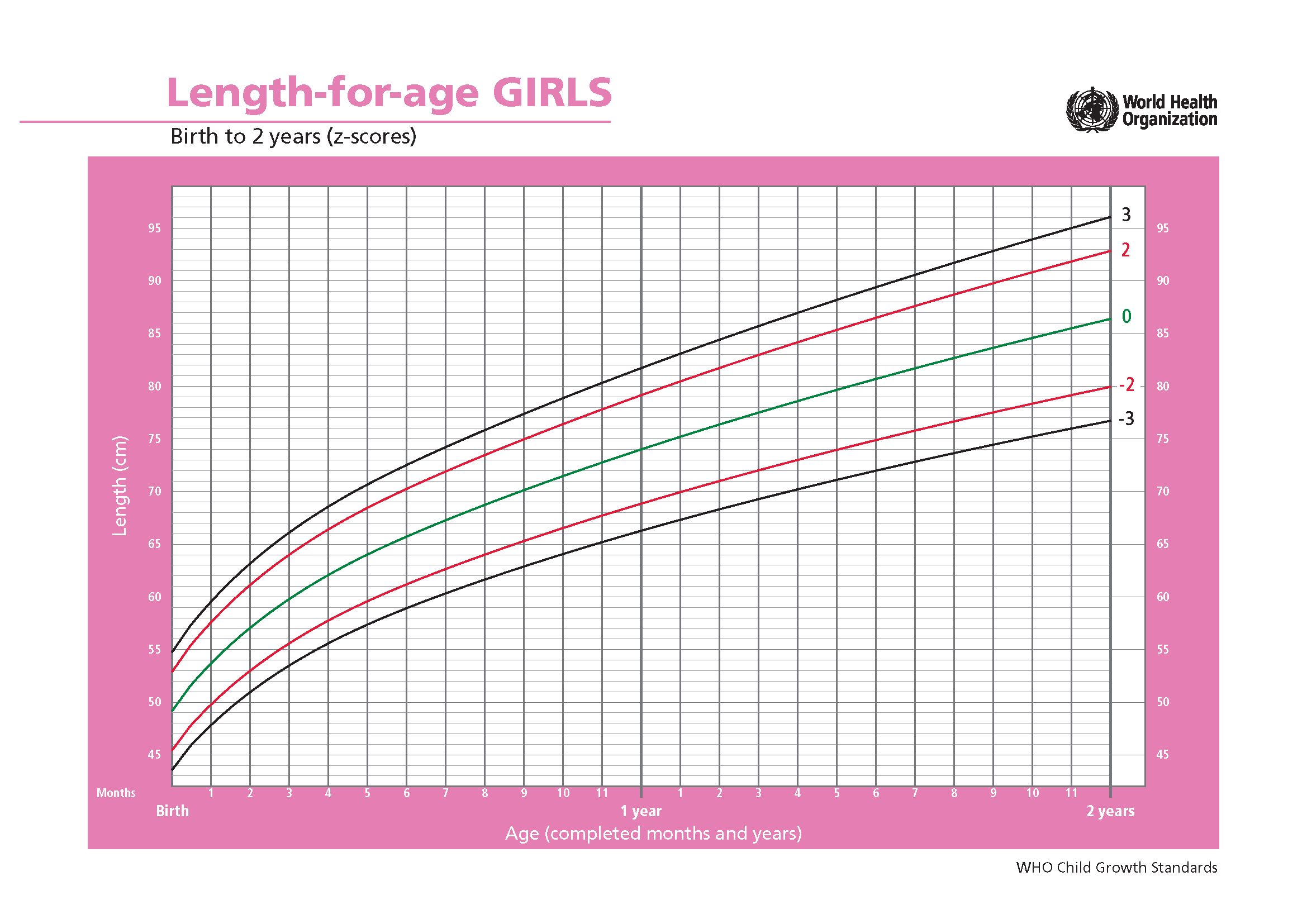{#fig-length-for-age-girls}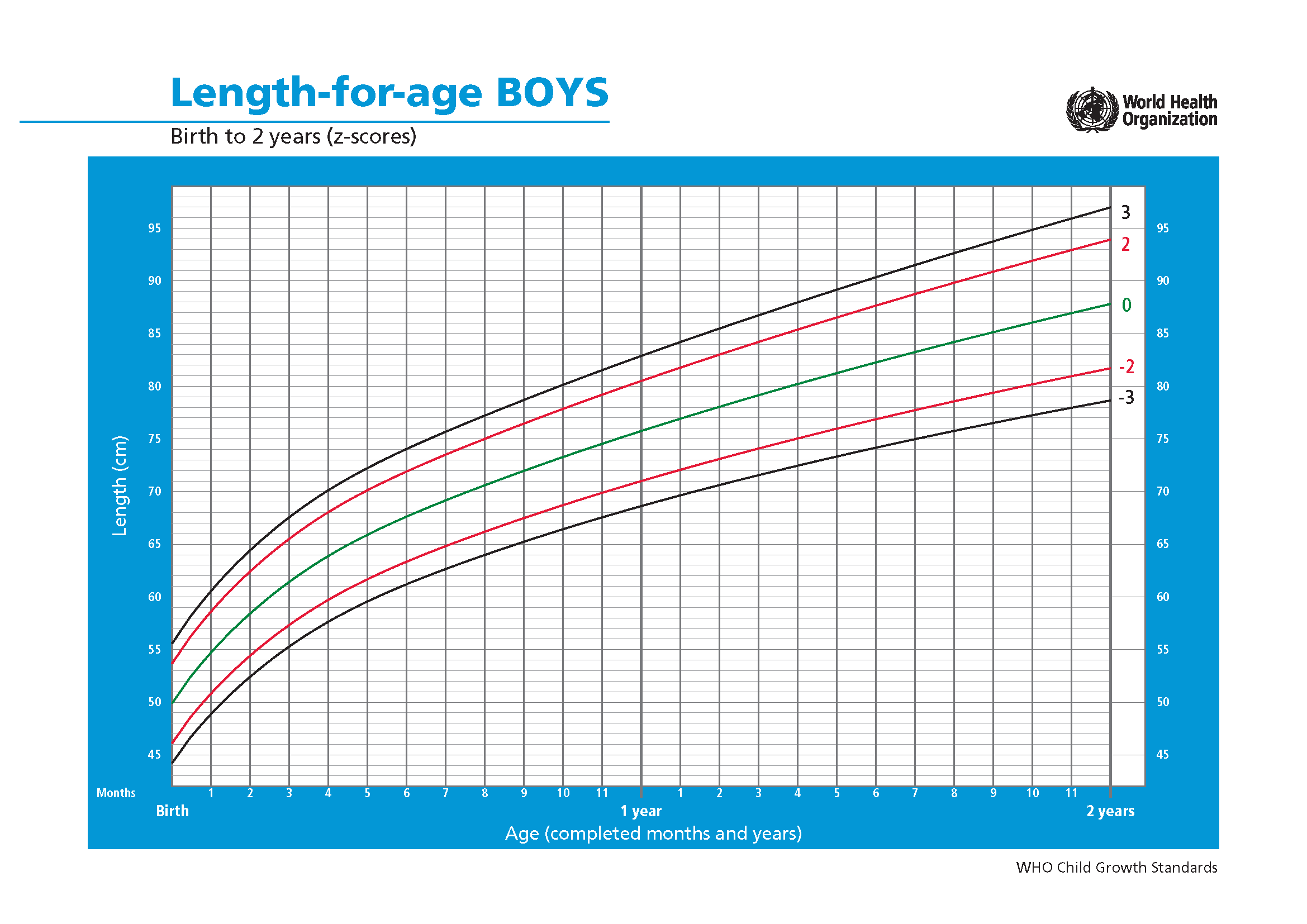{#fig-length-for-age-boys}Z-scores for the length-to-age ratio for girls and boys aged 0 to 2 years. Source: WHO. **Click on the images to enlargen them.**:::::: {.callout-task}3. Based on the dataset imported, calculate mean and standard deviation for the girls and the boys, how does it relate to the data from WHO?:::You can use the command `X <- X[complete.cases(X),]` to remove the empty rows in the dataframe `X`, or google how to compute descriptive statistics in the case of missing values. ::: {.callout-task}4. What is the Z-value? How can you use it to relate the dataset to the WHO data?5. Calculate the Z-scores for all the boys and girls.:::This can be done by creating a new vector inserting the length-vector from the previous dataframe to the equation for Z-score.::: {.callout-task}6. What does it mean that a child is above or below 0 in Z-score? How many children has a Z-score below -2 and -3?7. How many children are longer/taller than the world average? 8. Investigate whether some of the other variables (source of water *primary_watersource* or treatment of water *water_treatment_type*) impact the length at 15 months. Use `ggplot()` to do the plotting, and then use `ggplot(...) + facet_wrap(~SEX)` to split the plot in two corresponding to the variable *SEX*. Are the trends similar for the two sexes?::::::