17 Analysis of Variance (ANOVA)

Learning objectives

The learning objectives for this theme is to understand the statistical comparison of means from e.g. several different treatments. That is:

ANOVA is based on separation of the total variance in the data.
The inferential test is relating the systematic variance with the random variance.
To grasp, that the ratio of variances can be tested in a F-distribution.
Be able to compare responses to several ”treatments”, by model specification, hypothesis formulation and testing.
Be able to validate model assumptions.
To understand the relation between t-test and one-way ANOVA, and use a one-way ANOVA model to do pairwise comparisons between treatment 1 and treatment 2, treatment 1 and treatment 3, and so forth.
To be able to compute anova with one or two factors.

In short, ANOVA can be seen as an extention of the t-test. One-way ANOVA is for two sample t-test with more than two samples. And two-way anova is for paired t-test where there are more than just a pair.

17.1 Reading material

Analysis of Variance (ANOVA) - in short
A brief video going through the concepts of both one-way and two-way ANOVA:
- Analysis of Variance (ANOVA)
A video going through how to do ANOVA in R:
- ANOVA in R
Chapter 8 of Introduction to Statistics by Brockhoff

17.2 Analysis of Variance (ANOVA) - in short

17.2.1 Model formulation

Depending on the notes, there are several ways to write up the data for an ANOVA model. The following three versions are exactly similar for a setup with $k$ groups, and possibly not equal number of observations within each group. \

Version 1: \[\begin{aligned} X_{11},X_{12},X_{13},...,X_{1n_1} &\sim \mathcal{N}(\mu_1,\sigma^2) \\ X_{21},X_{22},X_{23},...,X_{2n_2} &\sim \mathcal{N}(\mu_2,\sigma^2) \\ & \vdots \\ X_{k1},X_{k2},X_{k3},...,X_{kn_k} &\sim \mathcal{N}(\mu_k,\sigma^2) \end{aligned}\]

Version 2: \[\begin{gather} X_{ij}\sim \mathcal{N}(\mu_i,\sigma^2)\\ \text{for } j=1,...,n_i \text{ and } i=1,..,k \nonumber \end{gather}\]

Version 3: \[\begin{gather} X_{ij} = \mu_i + e_{ij} \nonumber \\ \text{where } e_{ij}\sim \mathcal{N}(0,\sigma^2) \text{ and independent} \\ \text{for } j=1,...,n_i \text {and } i=1,..,k \nonumber \end{gather}\]

For all three versions, the parameters describing the groups ($\mu_i$ for $i=1,..,k$) and the dispersion within the groups ($\sigma$) appear, and are exactly similar. Naturally, all three versions are correct, but in order to harmonize with notation for ANOVA with several factors and regression we stick with version 3.

For these models it is assumed that the residuals are coming from the same normal distribution. That is: $e_{ij}\sim \mathcal{N}(0,\sigma^2)$. By construction, this distribution has mean equal to zero. Further it is assumed that these residuals are independent, that is: Changing one will not affect the others. If these two assumptions (same distribution and independent) are not fulfilled, the model is not valid, and we cannot trust the tests. Therefor this is checked by visual inspection of the residuals for normality (qq-plot, histogram, residuals vs. predicted value etc.) and independence (residuals vs. predicted value, line-plotting). As this is a very inherent part of model validation, it is made easy in R, where plot() on the object created by aov() or lm() produces graphics which can be used directly; fast’n’easy.

17.2.2 Hypothesis

$\mu_1,..,\mu_k$ describes the center of each of the $1,..,k$ samples, and is naturally what is interesting to compare. Usually we are looking for differences between these means, why the null hypothesis is:

\[\begin{equation} H0: \mu_1 = \mu_2 = ... = \mu_k \end{equation}\]

with the alternative, that at least one group .

17.2.3 ANOVA table and test

If we have two groups, the natural choice would be to use the differences between the observed means. However, for $k$ groups there are $k(k-1)/2$ combinations, why this approach would not lead to a single test, but merely $k(k-1)/2$ comparisons.

As an alternative for the differences between the observed means $\bar{X}_1,...,\bar{X}_k$, the variance across these numbers are used (only totally true for groups of equal size), that is: $MS_{bewteen} = var(\bar{X}_1,...,\bar{X}_k)$. If there is large differences between the group means, then this measure $MS_{bewteen}$ is big, and the null hypothesis should be discarded. Formalized, this needs to be compared to the variance within the groups, that is the average spread around the points.

It turns out, that this process can be seen as a partitioning (splitting) of the total variance in the entire dataset into

how much can be ascribed to the fact that samples are from different groups, and
how much which is caused by natural variation within the groups.

A natural way to organize these variances is in an ANOVA table. That is a table including the Sum of Squares (SSQ), Degrees of Freedom (DF), Mean Square (MS), observed F-statistic ($F_{obs}$ ), and $p$-value for each F-statistic $Pr(F_{df_A,df_e}>F_{obs})$. table 17.1 corresponds to a one-way ANOVA table (an analysis with one factor).

Table 17.1: ANOVA table for one-way analysis of variance.

Source	SSQ	DF	MS	$F_{obs}$	$Pr(F_{df_A,df_e}>F_{obs})$
Factor(A)	$SS_A$	$df_A = k-1$	$MS_A = SS_A/df_A$	$F_A = MS_A/MS_e$	$p_A$
Residuals	$SS_e$	$df_e = n-k$	$MS_e = SS_e/df_e$
Total	$SS_{tot}$	$df_{tot} = n-1$

Here the total variance is described as the sums of squares across all samples

\[ SS_{tot} = \sum{(X_{ij} - \bar{\bar{X}})^2} \quad \text{for all} \quad j=1,...,n_i, \text{ and } i = 1,..,k, \]

where $\bar{\bar{X}}$ is the overall average and $X_{ij}$ is the individual observations.

In the columns Sum of squares and Degrees of freedom, is the sum of the elements.

In the two sample t-test we use the pooled variance $s_{X_{pooled}}^2$, In ANOVA this number is reflected by the residual variation $MS_e$, which is also the estimate of $\sigma^2$ (I.e. $\hat{\sigma}^2 = MS_e$).

17.2.4 ANOVA with several factors

Experiments often consist of several factors. For instance Coffee served at different Temperatures evaluated by different Judges, beer produced from different Hops and different Yeast cultures or oil stored at different Temperature, over Time, at different Oxygen levels and different Light conditions.

Model

Imagine an experiment with two factors: $A$ and $B$, where $A$ has two levels, and $B$ has three levels, then the model is simply an extension of the one-way model:

\[\begin{gather} X_{i} = \alpha(A_i) + \beta(B_i) + e_{i} \nonumber \\ \text{where } e_{i}\sim \mathcal{N}(0,\sigma^2) \text{ and independent} \\ \text{for } i=1,...,n \nonumber \end{gather}\]

In this equation, $\alpha()$ describes the level with respect to $A$, and has two levels: $\alpha(A=1)$ and $\alpha(A=2)$, and $\beta()$ describes the level with respect to $B$, and has three levels: $\beta(B=1)$, $\beta(B=2)$ and $\beta(B=3)$.

Hypotheses

The associated null hypothesis are:

Factor A: $H0: \alpha(A=1) = \alpha(A=2)= .... = \alpha(A=k_A)$
Factor B: $H0: \beta(B=1) = \beta(B=2)= .... = \beta(B=k_B)$

ANOVA table

In the test of these hypothesis, the ANOVA table is simply extend with rows in relation to these effects table 17.2.

Table 17.2: ANOVA table for a two-way ANOVA.

Source	SSQ	DF	MS	$F_{obs}$	$Pr(F_{df_{Source},df_e}>F_{obs})$
Factor(A)	$SS_A$	$df_A = k_A-1$	$MS_A = SS_A/df_A$	$F_A = MS_A/MS_e$	$p_A$
Factor(B)	$SS_B$	$df_B = k_B-1$	$MS_B = SS_B/df_B$	$F_B = MS_B/MS_e$	$p_B$
Residuals	$SS_e$	$df_e = n-df_A - df_B - 1$	$MS_e = SS_e/df_e$
Total	$SS_{tot}$	$df_{tot} = n-1$

Interactions

For some experiments the effect of one factor might be dependent on the other factor, that is referred to as interaction. The interaction model for a two factor experiment is written as:

\[\begin{gather} X_{i} = \alpha(A_i) + \beta(B_i) + \gamma(A_i,B_i) + e_{i} \nonumber \\ \text{where } e_{i}\sim \mathcal{N}(0,\sigma^2) \text{ and independent} \\ \text{for } j=1,...,n \nonumber \end{gather}\]

where $\gamma()$ describes the interaction between the two factor. In a model with e.g. $2$ and $3$ levels for the factors, this interaction term naturally has $2\cdot 3 = 6$ levels. However, in the model above, the main effects ($\alpha$ and $\beta$) are included, so that consumes some of the levels. Actually, this factor has $(k_A - 1)(k_B - 1)$ levels.

ANOVA table - interactions

Testing the interaction leads to an extension of the ANOVA table, as seen in table 17.3.

Table 17.3: ANOVA table for a two-way ANOVA with interaction.

Source	SSQ	DF	MS	$F_{obs}$	$Pr(F_{df_{Source},df_e}>F_{obs})$
Factor(A)	$SS_A$	$df_A = k_A-1$	$MS_A = SS_A/df_A$	$F_A = MS_A/MS_e$	$p_A$
Factor(B)	$SS_B$	$df_B = k_B-1$	$MS_B = SS_B/df_B$	$F_B = MS_B/MS_e$	$p_B$
Factor(A*B)	$SS_{AB}$	$df_{AB} = (k_A-1)(k_B-1)$	$MS_{AB} = SS_{AB}/df_{AB}$	$F_{AB} = MS_{AB}/MS_e$	$p_{AB}$
Residuals	$SS_e$	$df_e = n-df_A - df_B - df_{AB} - 1 = n - (k_A)(k_B)$	$MS_e = SS_e/df_e$
Total	$SS_{tot}$	$df_{tot} = n-1$

We see that the only thing that changes is the sums of squares and the degrees of freedom for the residuals.

Example 17.1

Example 17.1 - Natural phenolic antioxidants for meat preservation - ANOVA

This example is based on the sensory data on the meat sausages treated with green tea (GT) and rosemary extract (RE) or control, used previously in example @#exa-natural-phenolic-antiox-paired-t-test.

A two-way anova can be used to evaluate the effect of several factors, and possible interaction effects on a single response variable. Here, we define a model with systematic effects of Treatment (3 levels), Assessor (8 levels) and Week (2 levels). Since it may be that the effect of the storage time differs for each of the antioxidant treatments, an interaciton effect between Treatment and Week is also included.

The starting model is therefore formulated as:

\[\begin{equation} Y_i=\alpha (Treat_i)+\beta(Assessor_i)+\gamma(Week_i)+\theta(Treat_i\times Week_i)+e_i \end{equation}\]

where $e_i \sim \mathcal{N}(0,\sigma ^2)$ and independent for $i=1,\ldots,n$

Plot the data

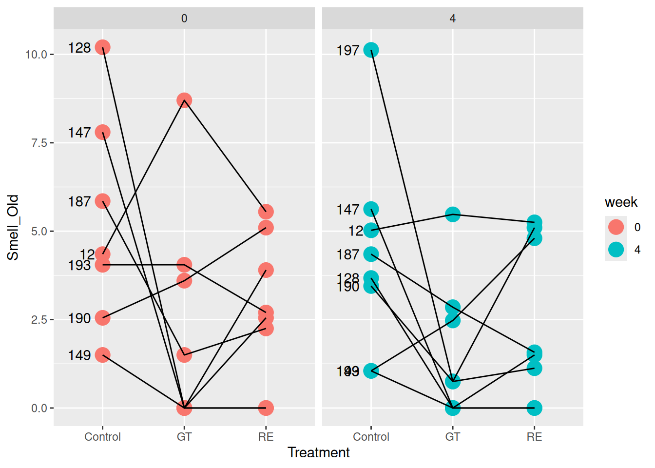
We wish to visualize three factors on a single response variable (figure 17.1). Here we use the x-axis for Week and Treatment, whereas the points are connected within Assessor.

ggplot(X, aes(Treatment, Smell_Old, group = Assessor)) +
  geom_point(size = 5, aes(color = week)) +
  geom_line() +
  facet_wrap(~week) +
  geom_text(
    data = X[X$Treatment == "Control", ],
    aes(label = Assessor), 
    hjust = 1.5 # Move the labels a little to the left
  )

Figure 17.1: Feedback on *Smell_Old* for all judges as a function of treatment. The plot is divided into week 0 and week 4.

From the figure there are a few observations: First, some assessors (e.g.~128 and 197) use the entire range whereas some only scores in a narrow range (e.g.~12, 193 and 187). Generally it seems as the control treatment (at both time points) obtain higher scores compared to the treated samples. There are no apparent indications for the two treatments being different.

# Compute ANOVA using specified model:
# Smell_Old = Assessor + Treatment + Week + Treatment * Week
fit <- aov(Smell_Old ~ factor(Assessor) + factor(Treatment) * factor(week),
           data = X)

# Show ANOVA table
anova(fit)

Analysis of Variance Table

Response: Smell_Old
                               Df  Sum Sq Mean Sq F value   Pr(>F)   
factor(Assessor)                7  77.833  11.119  1.9861 0.086116 . 
factor(Treatment)               2  70.153  35.077  6.2653 0.004826 **
factor(week)                    1   5.629   5.629  1.0054 0.323084   
factor(Treatment):factor(week)  2   1.062   0.531  0.0948 0.909763   
Residuals                      34 190.352   5.599                    
---
Signif. codes:  0 '***' 0.001 '**' 0.01 '*' 0.05 '.' 0.1 ' ' 1

Important! The factor() calls are important as they convert the variables from numeric/strings to factors. What happens if you remove factor()?

# Turn column "Assessor", "Treatment" and "week" into factors
X <- X |> 
  mutate(across(c(Assessor, Treatment, week), factor))

# Compute ANOVA using specified model:
# Smell_Old = Assessor + Treatment + Week + Treatment * Week
fit <- aov(Smell_Old ~ Assessor + Treatment * week,
           data = X)

# Show ANOVA table
anova(fit)

Analysis of Variance Table

Response: Smell_Old
               Df  Sum Sq Mean Sq F value   Pr(>F)   
Assessor        7  77.833  11.119  1.9861 0.086116 . 
Treatment       2  70.153  35.077  6.2653 0.004826 **
week            1   5.629   5.629  1.0054 0.323084   
Treatment:week  2   1.062   0.531  0.0948 0.909763   
Residuals      34 190.352   5.599                    
---
Signif. codes:  0 '***' 0.001 '**' 0.01 '*' 0.05 '.' 0.1 ' ' 1

Here it can be seen that the only effect which is found significant ($p < 0.05$) for the Old_Smell response is the Treatment factor. No significance was found for the Week or interaction factors. The Assessor effect is not strictly signifcant, but on the borderline ($p=0.09$). If we plot the raw data (figure 17.1), it seems each of the assesors have different base levels of scoring the old smell descriptor. Therefore, it is chosen to keep the systematic effect of Assessor in the model. Furthermore, it can be seen that there is some variation in the Assessor evaluation of the treatment effect (non-parallel), indicating that the sensory panel is not very precise, and may be poorly trained.

Final model

The final model is therefore the model only including the effects of the treatment and Assessor factors:

\[\begin{equation} Y_i=\alpha (Treat_i)+\beta(Assessor_i)+e_i \end{equation}\]

where $e_i \sim \mathcal{N}(0,\sigma^2)$ and independent for $i=1,\ldots,n$.

The estimates for the factors ($\alpha(Control),\alpha(GT), \alpha(RE), \beta(Ass12),\ldots,\beta(193)$) as well as the standard deviation ($\hat{\sigma}$) can be obtained by first calculating a new model including only significant terms followed by the anova() and summary() commands.

17.2.5 Contrasts

If it turns out that there is a significant effect of the factor, a natural next step is to compare the individual levels by estimation of confidence intervals and/or testing differences. This is quite similar to comparing two means by t-test. The only difference is, that $\hat{\sigma}^2 = MS_e$ is used as the measure of random uncertainty (instead of $s_{X_{pooled}}^2$), and the degrees of freedom is NOT $n_1 + n_2 - 2$, but the degrees of freedom associated with the uncertainty estimate: $df_e$. Apart from that, the method is similar.

Assume that Factor(A) has five levels, then the comparison of e.g. level $2$ and $5$ is done as follows:

Confidence intervals

\[\begin{equation} \bar{X_5} - \bar{X_2} \pm t_{1 - \alpha/2,df_e}\sqrt{MS_e}\sqrt{\frac{1}{n_5} + \frac{1}{n_2}} \end{equation}\]

Where $t_{1 - \alpha/2,df_e}$ is the t-fractile at a user-specified level $\alpha$ with $df_e$ degrees of freedom.

Test of contrast

The associated hypothesis are stated as:

\[\begin{equation} H_0: \mu_5=\mu_2 \end{equation}\]

With the alternative:

\[\begin{equation} H_A: \mu_5 \neq \mu_2 \end{equation}\]

Then the test statistics is calculated as: \[\begin{equation} t_{obs} = \frac{\bar{X_5} - \bar{X_2}} {\sqrt{MS_e}\sqrt{\frac{1}{n_5} + \frac{1}{n_2}}} \end{equation}\] With the associated (2-sided) p-value: $p = 2 \cdot P(\mathcal{T}_{df=df_e}>t_{obs})$.

Example 17.2

Example 17.2 - Natural phenolic antioxidants for meat preservation - contrasts

In this example, we wish to compare pairs of levels within a factor from an ANOVA model. In Example 17.1 the Treatment effect from a two way model as shown below is significant, however, that does not imply that all levels are different, but only that at least a single strikes out.

We start by computing the ANOVA and assigning it to the variable fit.

# Compute ANOVA
fit <- aov(Smell_Old ~ factor(Assessor) + factor(Treatment),
           data = X)

# Print ANOVA table
anova(fit)

Analysis of Variance Table

Response: Smell_Old
                  Df  Sum Sq Mean Sq F value   Pr(>F)   
factor(Assessor)   7  77.833  11.119  2.0879 0.069457 . 
factor(Treatment)  2  70.153  35.077  6.5866 0.003573 **
Residuals         37 197.043   5.325                    
---
Signif. codes:  0 '***' 0.001 '**' 0.01 '*' 0.05 '.' 0.1 ' ' 1

We can use model.tables() to get means for each level of each factor.

# Show means across both factors
model.tables(fit, type = "means")

Tables of means
Grand mean
         
3.025532 

 factor(Assessor) 
       12   128   147 149   187   190   193   197
    5.725 2.312 2.237 1.1 3.062 2.763 3.187 3.975
rep 6.000 6.000 6.000 6.0 6.000 6.000 6.000 5.000

 factor(Treatment) 
    Control     GT     RE
      4.752  1.865  2.568
rep  15.000 16.000 16.000

The rows of numbers contain the means across each level. rep is the number of observations.

Contrasts

We wish to compare the treatments RE and GT. This a basically a two sample t-test, just where the entire dataset and model is used to calculate the standard deviation.

The hypothesis are: \[ H_0: \mu_{GT}=\mu_{RE} \quad \text{and} \quad H_A: \mu_{GT} \neq \mu_{RE} \]

Naturally, the driver of this test is the observed difference between the two means. In total the test-statistics amount to:

\[\begin{equation} t_{obs} = \frac{\bar{X}_{GT} - \bar{X}_{RE}} {\sqrt{MS_e}\sqrt{\frac{1}{n_{GT}} + \frac{1}{n_{RE}}}} \end{equation}\]

With the associated (2-sided) p-value:

\[ p = 2 \cdot P(\mathcal{T}_{df=df_e}>t_{obs}) \]

m1 <- 1.86 # GT mean
m2 <- 2.57 # RE mean
n1 <- 16 # GT n
n2 <- 16 # RE n
s <- sqrt(5.325) # SD from ANOVA table
df <- 37 # DF for residuals
t_obs <- (m1 - m2) / (s*sqrt(1/n1 + 1/n2)) # Test statistic
2*(1 - pt(abs(t_obs),df)) # p-value for GT vs RE

[1] 0.3897755

In line with the raw data, the observed difference between the two treatments, is not statistically singificant, and we conclude that the two treatments has similar properties in terms of Old_Smell.

Confidence interval on difference between RE and Control

As an alternative, the confidence interval on the difference between two means can be calculated. As example this is done for RE vs Control.

m3 <- 4.75 # Control mean
n3 <- 15 # Control n
CIlow <- m3 - m2 - qt(0.975,df)*s*sqrt(1/n2 + 1/n3) # lower bound
CIhigh <- m3 - m2 + qt(0.975,df)*s*sqrt(1/n2 + 1/n3) # upper bound
c(CIlow,CIhigh)

[1] 0.4995882 3.8604118

We see that the confidence interval on the difference between the control and RE treated samples are positive and do not overlap $0$, that is, in general the control samples has a higher score with respect to Old_Smell and further that this is a significant difference on $95\%$ level.

17.3 Videos

17.3.1 Analysis of Variance (ANOVA) - J David Eisenberg

17.3.2 Anova in R - Ed Boone

17.4 Exercises

17.4.1 ANOVA

Load Results panel.xlsx. Look at the study design and:

Tasks

Formulate a One-way ANOVA model for the coffees served at different Temperatures and the response bitter.
Formulate null-hypothesis and alternative hypothesis between the different coffee temperatures.
Test the hypothesis.
Formulate a Two-way ANOVA model for the taste of bitter with the two factors; Temperature and Judge
Formulate null-hypothesis and alternative hypothesis.

Exercise 17.1

Exercise 17.2

Exercise 17.1 - Wine and one-way ANOVA

Wines from four different countries (Argentina, Australia, Chile and South Africa) were analyzed for aroma compounds with GC-MS (gas chromatography coupled with mass spectrometry). The dataset can be found in the file “Wine.xlsx”. The wine data should already be familiar to you otherwise look at the exercises from week 1 and 2.

Tasks

When working with ANOVA which assumption is then made about the data, and how does the model look?
We would like to investigate if the wines from the four different countries are different. State the null hypothesis and the alternative hypothesis.
Make a combined jitter and boxplot on the variable X3.Hexenol. Are there any suspicious samples?
Make an ANOVA on X3.Hexenol, look at the summary() and draw conclusions.
Compare the result with the boxplot from Q3. Was the result of the ANOVA expected? If yes; why?
We would like to state which countries are significantly different from the others. For this you need to install the R-package multcomp. Use the command TukeyHSD() to investigate the differences/contrasts between the countries. Use the confidence intervals for judging differences.
Which countries are significantly different and which are not? Compare with the boxplot produced in Q3.
Make the boxplot and the ANOVA for the following variables too; Diethyl.succinate, X1.Hexanol, Ethyl.hexanoate and Ethyl.propanoate. Are any of these variables different between countries?
Check for normality of the model residuals by making a qq-plot.
- Hint: You need to extract the residuals from the model, for instance by the function resid(). Use qqnorm() and qqline() to make the plot.
1. Can we trust the assumption about normality?
2. After doing this manually, try the function plot() on the aov() object, which produces four plots for assumption checking.
For some of the results, the jitter plot indicates, a few extreme samples. What happens if these are removed? Does the conclusions change?

Exercise 17.3

Exercise 17.2 - Diet and fat metabolism - ANOVA

The diet is a central factor involved in general health, and especially in relation to obesity, where a balance between intake of protein, fat and carbohydrates, as well as types of these nutrients seems important. Therefore various controlled studies are conducted to show the effect of different diets. A study examining the effect of protein from milk (casein or whey) and amount of fat on growth biomarkers of fat metabolism and type I diabetes was conducted in 40 mice over an intervention period of 14 weeks.

The data for this exercise is the same as for Exercise 10.3.

For this exercise we are going to focus on cholesterol as a biomarker related to fat metabolism, and on three types of diet:

High fat with the milk protein casein HF casein (n=15).
High fat with whey protein from milk HF whey (n=15).
Low fat with the milk protein casein LF casein (n=10).

The cholesterol level at the end of the 14 week intervention is listed in table 17.4 including some descriptive stats.

Table 17.4: Some summary statistics for cholesterol across the three diets.

	1	2	…	9	10	11	…	15	$\sum{X}$	$\sum{(X - \bar{X})^2}$
Cholesterol (HF casein)	4.68	3.60	…	4.60	4.84	4.84	…	4.37	67.29	4.06
Cholesterol (HF whey)	3.79	2.82	…	3.77	4.63	3.44	…	3.24	54.86	4.69
Cholesterol (LF casein)	3.97	3.69	…	3.62	3.53	…	…	…	34.37	2.07

The total sums of squares is: $SS_{tot} = \sum{(X_{ij} - \bar{\bar{X}})^2} = 18.99$.

The first six questions are supposed to be done by hand where the computer only is used as a pocket calculator.

Tasks

Calculate descriptive statistics for the three groups
- Hint: Fill in the table the missing values in table 17.4.
Sketch these results in a graph (by pen and paper - no computer).
State a model for these data, and a hypothesis of similarity between the three dietary treatments (with regards to cholesterol level).
Construct an ANOVA table and calculate and fill in the numbers including test statistics ($F_{obs}$) and the corresponding p-value.
- For the translation of $F_{obs}$ to $p$, use the function pf() in R.
This p-value should be significant. Guided by the initial descriptive stats, do you believe that all three diets are different? Or is there two groups which are close in estimate?
Formulate a hypothesis of similarity between the two most similar groups. Test this contrast.

The data can be found in the file Mouse_diet_intervention.xlsx.

Tasks

Import the data, and make a plot of cholesterol ($cholesterol) and dietary intervention ($Fat_Protein)
Repeat the ANOVA analysis using R with the function aov() for construction of model and the function anova() for analysis of this model.
Check that the model assumptions are ok.
- plot(model) where model is the object created by aov().
For the individual contrasts you can use the function TukeyHSD() on the model.
- Be aware that the p-values in this analysis is adjusted for multiple testing, and therefore are bigger than the ones done one by one.
Based on these results, which dietary component do you think causes differences in cholesterol level?
There are some indications of differences between HF whey and LF casein, however, not significant. How many samples would have been needed in order to achieve significance with an appropriate power level?

Exercise 17.4

Exercise 17.3 - Diet and fat metabolism - multivariate ANOVA

In this exercise, we are going to extend the analysis from Exercise 17.3 to include several biomarkers.

Tasks

Start out by construction of a PCA on the biomarkers: insulin, cholesterol, triglycerides, NEFA, glucose and HbA1c (NEFA = nonesterified fatty acids), including all 40 samples, and comment on the results with respect to differences between diets. This is computationally identical to the task in Exercise 10.3.
Repeat the ANOVA for several biomarkers including plotting.
Zack out the components in the PCA model and glue them together with the original data (use cbind()).
- You can find inspiration on how to do this in Exercise 6.1.
Use the components from the PCA model as response variables, and repeat the ANOVA (including plotting).
Comment on the similarity / dis-similarity between the univariate results, and the ones based on the PCA.
Compare the results (plot and ANOVA) for PC1 and PC6. Why do you think the dietary signal is more pronounced in the first component?
- Hint: Think of how much, and which type of variation that is captured in the individual components.

Exercise 17.5

Exercise 17.4 - Analysis of coffee serving temperature

Serving temperature of coffee seems of importance of how this drink is perceived. However, it is not totally clear how this relation is. In order to understand this, studies on the same type of coffee served at different temperature is conducted. In this exercise we are going to use the data from a trained Panel of eight judges, evaluating coffee served at six different temperatures on a set of sensorical descriptors. Each judge is presented with each temperature in a total of four replicates leading to a total of $6 \times 8 \times 4 = 192$ samples.

In the dataset Results Panel.xlsx the results are listed. In this exercise we are going to analyse the differences between the individual temperatures while utilizing the design of repeated scoring by the same judges. This exercise is an extension of Exercise 6.2 from week one.

Tasks

We want to summarize data, such that each judge have one score for each coffee sample and each attribute (instead of four).
- You can use the aggregate() function to average over replicates, which is to retain Assessor and Sample.
Plot this descriptive measure for Intensity across temperature (x-axis) and join the points from the same judge.
Make an ANOVA model with the response Intensity including both factors (Temperature and Judge).
Check out what the function factor() is doing? What happens if it is removed (check the degrees of freedoms consumed by the two options).
Check that the model assumptions are ok. (plot(model) where model is the object created by aov()).
Comment on these results (in relation to Temperature and Judge).
Use this data as input for construction of a PCA model, and make a bi-plot.
What do you see with respect to differences in temperature and judges?
Zack out the first couple of component and glue them together with the original data.
Make ANOVA model for component 1 to 5 and find the component with the strongest Temperature and Judge signature respectively.
Plot the PCA model with these two components (This is specified by the option choice = ...). Color this plot according to Temperature and Judge.
Which sensorical markers seems mostly related to differences between Temperature and Judge respectively?

Exercise 17.6

Exercise 17.5 - Carcass suspension

Toughness is found to be the most important quality characteristic in beef. Variation in toughness is primarily related to the muscle fibers and the connective tissue. Connective tissue is thought to be responsible for the relative fixed background toughness, largely affected by animal age. The toughness of the muscle fibers depends on a couple of factors and is more likely to be manipulated by e.g. carcass suspension to prevent post-mortem contraction of the muscle fibers.

An experiment was conducted in order to test the effects of Animal Age, Carcass Suspension and the interaction between Animal Age and Carcass Suspension. The muscle of interest was longissimus dorsi. The hypothesis for the experiment was that pelvic suspension would prevent post-mortem contraction of the muscle fibers and thereby result in a more tender longissimus dorsi compared with suspension in the Achilles tendon. Furthermore, the toughness was believed to increase with increasing age. This increase in toughness was assigned to connective tissue.

In the experiment, animals were slaughtered and the carcasses were spilt. One side was suspended in in the pelvic bone (figure 17.2, left) and the other side was suspended in the Achilles tendon (figure 17.2, right). The experiment was balanced and 15 carcass sides were assigned to each group.

Figure 17.2: Left: Pelvic suspension. Right: Achilles suspension.

In the table 17.5 are shown the average results from each cell in the design.

Table 17.5: Mean values for the design (n = 15 in each group)

Suspension	Age 2y	Age 3y	Age 4y
Pelvic (A)	58.5	65.0	66.0
Achilles (B)	72.0	82.5	93.0

Tasks

Sketch these results with the response on the y-axis, one factor on the x-axis, and join the points based on the other factor. What is your first impression on the effect of age of the animal and of suspension method.
- Further, does the lines seem to be deviating from being parallel? (This indicates interaction between the factors).
Write up a model including interaction term.
Write up the $H0$ (and the alternative) hypotheses for the main effects in this experiment.

Table 17.6: ANOVA table for response shear force.

Source	SS	df	MS	F	p-value
Age	3083.7
Suspension	8410.0
Age*Suspension
Error			375.0	-	-
Total	43715.0	89	-	-	-

Tasks

Fill the missing values in the table 17.6.
What factors are having a significant effect (significance level of 0.05)?
Modify the two-way ANOVA model. Should the interaction be included in the final model for the present study? Why/Why not?
Toughness is explained by muscle fibers and connective tissue. The contribution from muscle fibers is impacted by suspension method. The contribution from connective tissue is impacted by age. Would you expect an effect of the interaction term between suspension method and age? Why/Why not? How does your answer correspond with the answers in question 6?
Traditionally, carcasses suspension is done by Achilles, what would you recommend based on this study? What are the limitations/assumptions for such a recommendation?
- Hint: Have we checked all muscles? Look at the picture - do you think the conclusions extrapolate to other parts of the animal?

Exercise 17.7

Exercise 17.6 - Stability of oil under different conditions

This exercise is a direct extension of Exercise 10.5.

Oil are primary made up of triglycerides, where some of the fatty acids are unsaturated. This causes such a product to be susceptible to oxidation both from chemical oxidative agents such as metal ions, or from exposure to light. Oxidation of the unsaturated fatty acids changes the sensorical and physical properties of the oil.

In the southern part of Africa grows a robust bean - the Marama bean. This bean has a favorable dietary composition, including dietary fibers, fats and proteins, as most similar types of nuts, therefore this crop could be utilized for making healthy products by the locals for the locals. One such product is Marama bean oil. A study has been conducted to investigate the oxidative stability of the oil under various conditions. In the dataset MaramaBeanOilOx.xlsx are listed the results from such an experiment (including data from both normal and roasted beans). The experimental factors are:

Storage time (Month)
Product type (Product)
Storage temperature (Temperature)
Storage condition (Light)
Packaging air (Air)

The response variable reflecting oxidative stability is peroxide value and named PV.

The first three questions are identical to Exercise 10.5.

Tasks

Read in the data, and subset so that you only include data related to product type Oil.
Make descriptive plots of the response variable PV imposing storage temperature, condition, and time.
- Hint: factor(Temperature):Light specifies all combinations of these two factors. facet_grid(.~Month) splits the plot into several plots according to Month.
What do you observe in terms of storage time, temperature and condition from this plot?
Based on the plot, suggest a model including the three factors Month, Temperature and Light. Which factors do you think is additive (i.e. have the same effect regardless of the other factors), and which do you think interacts?
Build a model including all combinations of the three factors.
- That is: m <- aov(data=Marama.oil, PV~factor(Temperature)*Light*factor(Month)).
Check the assumption concerning the distribution of the residuals. If necessary, make an appropriate transformation of the response variable, and check that it is doing better in terms of distributional assumptions for the model residuals.
It seems like we need all combinations of everything. Construct a single variable, that has the seven levels indicating the design, and use this in an ANOVA model.
- Hint: Allcomp <- factor(Marama.oil$Temperature):Marama.oil$Light:factor(Marama.oil$Month
Use TukeyHSD() on that model to make all pairwise comparisons of the seven individual levels. And comment on what you obtain. Does the initial plot correspond to the pairwise observations?

# Analysis of Variance (ANOVA) ```{r} #| label: anova-setup #| echo: false #| message: false #| warning: false library(ggplot2) library(dplyr) library(here) ``` ::: {.callout-tip} ## Learning objectives The learning objectives for this theme is to understand the statistical comparison of means from e.g. several different treatments. That is: * ANOVA is based on separation of the total variance in the data. * The inferential test is relating the systematic variance with the random variance. * To grasp, that the ratio of variances can be tested in a F-distribution. * Be able to compare responses to several ”treatments”, by model specification, hypothesis formulation and testing. * Be able to validate model assumptions. * To understand the relation between t-test and one-way ANOVA, and use a one-way ANOVA model to do pairwise comparisons between treatment 1 and treatment 2, treatment 1 and treatment 3, and so forth. * To be able to compute anova with one or two factors. In short, ANOVA can be seen as an extention of the t-test. One-way ANOVA is for two sample t-test with more than two samples. And two-way anova is for paired t-test where there are more than just a pair. ::: ## Reading material * [Analysis of Variance (ANOVA) - in short](#sec-anova-intro) * A brief video going through the concepts of both one-way and two-way ANOVA: * [Analysis of Variance (ANOVA)](#sec-anova-eisenberg) * A video going through how to do ANOVA in R: * [ANOVA in R](#sec-anova-boone) * Chapter 8 of [*Introduction to Statistics*](https://02402.compute.dtu.dk/enotes/book-IntroStatistics) by Brockhoff ## Analysis of Variance (ANOVA) - in short {#sec-anova-intro} ### Model formulation Depending on the notes, there are several ways to write up the data for an ANOVA model. The following three versions are exactly similar for a setup with $k$ groups, and possibly not equal number of observations within each group. \\ Version 1: \begin{aligned} X_{11},X_{12},X_{13},...,X_{1n_1} &\sim \mathcal{N}(\mu_1,\sigma^2) \\ X_{21},X_{22},X_{23},...,X_{2n_2} &\sim \mathcal{N}(\mu_2,\sigma^2) \\ & \vdots \\ X_{k1},X_{k2},X_{k3},...,X_{kn_k} &\sim \mathcal{N}(\mu_k,\sigma^2) \end{aligned} Version 2: \begin{gather} X_{ij}\sim \mathcal{N}(\mu_i,\sigma^2)\\ \text{for } j=1,...,n_i \text{ and } i=1,..,k \nonumber \end{gather} Version 3: \begin{gather} X_{ij} = \mu_i + e_{ij} \nonumber \\ \text{where } e_{ij}\sim \mathcal{N}(0,\sigma^2) \text{ and independent} \\ \text{for } j=1,...,n_i \text {and } i=1,..,k \nonumber \end{gather} For all three versions, the parameters describing the groups ($\mu_i$ for $i=1,..,k$) and the dispersion within the groups ($\sigma$) appear, and are exactly similar. Naturally, all three versions are correct, but in order to harmonize with notation for ANOVA with several factors and regression we stick with version 3. For these models it is assumed that the residuals are coming from the *same* normal distribution. That is: $e_{ij}\sim \mathcal{N}(0,\sigma^2)$. By construction, this distribution has mean equal to zero. Further it is assumed that these residuals are independent, that is: Changing one will not affect the others. If these two assumptions (same distribution and independent) are not fulfilled, the model is not valid, and we cannot trust the tests. Therefor this is checked by visual inspection of the residuals for normality (qq-plot, histogram, residuals vs. predicted value etc.) and independence (residuals vs. predicted value, line-plotting). As this is a very inherent part of model validation, it is made easy in R, where `plot()` on the object created by `aov()` or `lm()` produces graphics which can be used directly; fast'n'easy. ### Hypothesis $\mu_1,..,\mu_k$ describes the center of each of the $1,..,k$ samples, and is naturally what is interesting to compare. Usually we are looking for differences between these means, why the null hypothesis is: \begin{equation} H0: \mu_1 = \mu_2 = ... = \mu_k \end{equation} with the alternative, that at least one group \textit{sticks out}. ### ANOVA table and test If we have two groups, the natural choice would be to use the differences between the observed means. However, for $k$ groups there are $k(k-1)/2$ combinations, why this approach would not lead to a single test, but merely $k(k-1)/2$ comparisons. As an alternative for the differences between the observed means $\bar{X}_1,...,\bar{X}_k$, the variance across these numbers are used (only totally true for groups of equal size), that is: $MS_{bewteen} = var(\bar{X}_1,...,\bar{X}_k)$. If there is large differences between the group means, then this measure $MS_{bewteen}$ is big, and the null hypothesis should be discarded. Formalized, this needs to be compared to the variance within the groups, that is the average spread around the points. It turns out, that this process can be seen as a partitioning (splitting) of the total variance in the entire dataset into 1. how much can be ascribed to the fact that samples are from different groups, and 2. how much which is caused by natural variation within the groups. A natural way to organize these variances is in an ANOVA table. That is a table including the Sum of Squares (SSQ), Degrees of Freedom (DF), Mean Square (MS), observed F-statistic ($F_{obs}$ ), and $p$-value for each F-statistic $Pr(F_{df_A,df_e}>F_{obs})$. @tbl-one-way-anova corresponds to a one-way ANOVA table (an analysis with one factor). | Source | SSQ | DF | MS| $F_{obs}$ | $Pr(F_{df_A,df_e}>F_{obs})$ | |------------|----------|------------------|---------------------|-------------------|----------------------------| | Factor(A) | $SS_A$ | $df_A = k-1$ | $MS_A = SS_A/df_A$ | $F_A = MS_A/MS_e$ | $p_A$ | | Residuals | $SS_e$ | $df_e = n-k$ | $MS_e = SS_e/df_e$ | | | | Total | $SS_{tot}$ | $df_{tot} = n-1$ | | | | : ANOVA table for one-way analysis of variance. {#tbl-one-way-anova .hover .responsive} Here the total variance is described as the sums of squares across all samples $$ SS_{tot} = \sum{(X_{ij} - \bar{\bar{X}})^2} \quad \text{for all} \quad j=1,...,n_i, \text{ and } i = 1,..,k, $$ where $\bar{\bar{X}}$ is the overall average and $X_{ij}$ is the individual observations. In the columns *Sum of squares* and *Degrees of freedom*, is the sum of the elements. In the two sample t-test we use the pooled variance $s_{X_{pooled}}^2$, In ANOVA this number is reflected by the residual variation $MS_e$, which is also the estimate of $\sigma^2$ (I.e. $\hat{\sigma}^2 = MS_e$). ### ANOVA with several factors Experiments often consist of several factors. For instance Coffee served at different *Temperatures* evaluated by different *Judges*, beer produced from different *Hops* and different *Yeast cultures* or oil stored at different *Temperature*, over *Time*, at different *Oxygen levels* and different *Light conditions*. #### Model Imagine an experiment with two factors: $A$ and $B$, where $A$ has two levels, and $B$ has three levels, then the model is simply an extension of the one-way model: \begin{gather} X_{i} = \alpha(A_i) + \beta(B_i) + e_{i} \nonumber \\ \text{where } e_{i}\sim \mathcal{N}(0,\sigma^2) \text{ and independent} \\ \text{for } i=1,...,n \nonumber \end{gather} In this equation, $\alpha()$ describes the level with respect to $A$, and has two levels: $\alpha(A=1)$ and $\alpha(A=2)$, and $\beta()$ describes the level with respect to $B$, and has three levels: $\beta(B=1)$, $\beta(B=2)$ and $\beta(B=3)$. #### Hypotheses The associated null hypothesis are: * Factor A: $H0: \alpha(A=1) = \alpha(A=2)= .... = \alpha(A=k_A)$ * Factor B: $H0: \beta(B=1) = \beta(B=2)= .... = \beta(B=k_B)$ #### ANOVA table In the test of these hypothesis, the ANOVA table is simply extend with rows in relation to these effects @tbl-two-way-anova. | Source | SSQ | DF | MS | $F_{obs}$ | $Pr(F_{df_{Source},df_e}>F_{obs})$ | |------------|----------|------|-----------|------------|-----------------------------------| | Factor(A) | $SS_A$ | $df_A = k_A-1$ | $MS_A = SS_A/df_A$ | $F_A = MS_A/MS_e$ | $p_A$ | | Factor(B) | $SS_B$ | $df_B = k_B-1$ | $MS_B = SS_B/df_B$ | $F_B = MS_B/MS_e$ | $p_B$ | | Residuals | $SS_e$ | $df_e = n-df_A - df_B - 1$ | $MS_e = SS_e/df_e$ | | | | Total | $SS_{tot}$ | $df_{tot} = n-1$ | | | | : ANOVA table for a two-way ANOVA. {#tbl-two-way-anova .hover .responsive} #### Interactions For some experiments the effect of one factor might be dependent on the other factor, that is referred to as *interaction*. The interaction model for a two factor experiment is written as: \begin{gather} X_{i} = \alpha(A_i) + \beta(B_i) + \gamma(A_i,B_i) + e_{i} \nonumber \\ \text{where } e_{i}\sim \mathcal{N}(0,\sigma^2) \text{ and independent} \\ \text{for } j=1,...,n \nonumber \end{gather} where $\gamma()$ describes the interaction between the two factor. In a model with e.g. $2$ and $3$ levels for the factors, this interaction term naturally has $2\cdot 3 = 6$ levels. However, in the model above, the main effects ($\alpha$ and $\beta$) are included, so that consumes some of the levels. Actually, this factor has $(k_A - 1)(k_B - 1)$ levels. #### ANOVA table - interactions Testing the interaction leads to an extension of the ANOVA table, as seen in @tbl-two-way-anova-interaction. | Source | SSQ | DF | MS | $F_{obs}$ | $Pr(F_{df_{Source},df_e}>F_{obs})$ | |-------------|-----------|------------------------------------------------------------------|--------------------------|------------------------|-----------------------------------| | Factor(A) | $SS_A$ | $df_A = k_A-1$ | $MS_A = SS_A/df_A$ | $F_A = MS_A/MS_e$ | $p_A$ | | Factor(B) | $SS_B$ | $df_B = k_B-1$ | $MS_B = SS_B/df_B$ | $F_B = MS_B/MS_e$ | $p_B$ | | Factor(A*B) | $SS_{AB}$ | $df_{AB} = (k_A-1)(k_B-1)$ | $MS_{AB} = SS_{AB}/df_{AB}$ | $F_{AB} = MS_{AB}/MS_e$ | $p_{AB}$ | | Residuals | $SS_e$ | $df_e = n-df_A - df_B - df_{AB} - 1 = n - (k_A)(k_B)$ | $MS_e = SS_e/df_e$ | | | | Total | $SS_{tot}$ | $df_{tot} = n-1$ | | | | : ANOVA table for a two-way ANOVA with interaction. {#tbl-two-way-anova-interaction .hover .responsive} We see that the only thing that changes is the sums of squares and the degrees of freedom for the residuals. ::: {#exa-natural-phenolic-antiox-anova}  ::: ::: {.callout-example} ### Natural phenolic antioxidants for meat preservation - ANOVA ```{r} #| label: anova-example-setup #| echo: false #| message: false #| warning: false load(here("data", "meat_data.RData")) ``` This example is based on the sensory data on the meat sausages treated with green tea (GT) and rosemary extract (RE) or control, used previously in example @#exa-natural-phenolic-antiox-paired-t-test. A two-way anova can be used to evaluate the effect of several factors, and possible interaction effects on a single response variable. Here, we define a model with systematic effects of *Treatment* (3 levels), *Assessor* (8 levels) and *Week* (2 levels). Since it may be that the effect of the storage time differs for each of the antioxidant treatments, an interaciton effect between *Treatment* and *Week* is also included. The starting model is therefore formulated as: \begin{equation} Y_i=\alpha (Treat_i)+\beta(Assessor_i)+\gamma(Week_i)+\theta(Treat_i\times Week_i)+e_i \end{equation} where $e_i \sim \mathcal{N}(0,\sigma ^2)$ and independent for $i=1,\ldots,n$ #### Plot the data We wish to visualize three factors on a single response variable (@fig-smell-old-vs-treatment). Here we use the x-axis for *Week* and *Treatment*, whereas the points are connected within *Assessor*. ```{r} #| label: fig-smell-old-vs-treatment #| fig-cap: Feedback on *Smell_Old* for all judges as a function of treatment. The plot is divided into week 0 and week 4. ggplot(X, aes(Treatment, Smell_Old, group = Assessor)) + geom_point(size = 5, aes(color = week)) + geom_line() + facet_wrap(~week) + geom_text( data = X[X$Treatment == "Control", ], aes(label = Assessor), hjust = 1.5 # Move the labels a little to the left ) ``` From the figure there are a few observations: First, some assessors (e.g.~128 and 197) use the entire range whereas some only scores in a narrow range (e.g.~12, 193 and 187). Generally it seems as the control treatment (at both time points) obtain higher scores compared to the treated samples. There are no apparent indications for the two treatments being different. #### Calculate two-way ANOVA ::: {.panel-tabset} #### Using base R ```{r} # Compute ANOVA using specified model: # Smell_Old = Assessor + Treatment + Week + Treatment * Week fit <- aov(Smell_Old ~ factor(Assessor) + factor(Treatment) * factor(week), data = X) # Show ANOVA table anova(fit) ``` Important! The `factor()` calls are important as they convert the variables from numeric/strings to factors. What happens if you remove `factor()`? #### Using Tidyverse ```{r} # Turn column "Assessor", "Treatment" and "week" into factors X <- X |> mutate(across(c(Assessor, Treatment, week), factor)) # Compute ANOVA using specified model: # Smell_Old = Assessor + Treatment + Week + Treatment * Week fit <- aov(Smell_Old ~ Assessor + Treatment * week, data = X) # Show ANOVA table anova(fit) ``` ::: Here it can be seen that the only effect which is found significant ($p < 0.05$) for the *Old_Smell* response is the *Treatment* factor. No significance was found for the *Week* or interaction factors. The *Assessor* effect is not strictly signifcant, but on the borderline ($p=0.09$). If we plot the raw data (@fig-smell-old-vs-treatment), it seems each of the assesors have different base levels of scoring the old smell descriptor. Therefore, it is chosen to keep the systematic effect of *Assessor* in the model. Furthermore, it can be seen that there is some variation in the *Assessor* evaluation of the treatment effect (non-parallel), indicating that the sensory panel is not very precise, and may be poorly trained. #### Final model The final model is therefore the model only including the effects of the treatment and *Assessor* factors: \begin{equation} Y_i=\alpha (Treat_i)+\beta(Assessor_i)+e_i \end{equation} where $e_i \sim \mathcal{N}(0,\sigma^2)$ and independent for $i=1,\ldots,n$. The estimates for the factors ($\alpha(Control),\alpha(GT), \alpha(RE), \beta(Ass12),\ldots,\beta(193)$) as well as the standard deviation ($\hat{\sigma}$) can be obtained by first calculating a new model including only significant terms followed by the *anova()* and *summary()* commands. :::  ### Contrasts If it turns out that there is a significant effect of the factor, a natural next step is to compare the individual levels by estimation of confidence intervals and/or testing differences. This is quite similar to comparing two means by t-test. The only difference is, that $\hat{\sigma}^2 = MS_e$ is used as the measure of random uncertainty (instead of $s_{X_{pooled}}^2$), and the degrees of freedom is NOT $n_1 + n_2 - 2$, but the degrees of freedom associated with the uncertainty estimate: $df_e$. Apart from that, the method is similar. Assume that *Factor(A)* has five levels, then the comparison of e.g. level $2$ and $5$ is done as follows: #### Confidence intervals \begin{equation} \bar{X_5} - \bar{X_2} \pm t_{1 - \alpha/2,df_e}\sqrt{MS_e}\sqrt{\frac{1}{n_5} + \frac{1}{n_2}} \end{equation} Where $t_{1 - \alpha/2,df_e}$ is the t-fractile at a user-specified level $\alpha$ with $df_e$ degrees of freedom. #### Test of contrast The associated hypothesis are stated as: \begin{equation} H_0: \mu_5=\mu_2 \end{equation} With the alternative: \begin{equation} H_A: \mu_5 \neq \mu_2 \end{equation} Then the test statistics is calculated as: \begin{equation} t_{obs} = \frac{\bar{X_5} - \bar{X_2}} {\sqrt{MS_e}\sqrt{\frac{1}{n_5} + \frac{1}{n_2}}} \end{equation} With the associated (2-sided) p-value: $p = 2 \cdot P(\mathcal{T}_{df=df_e}>t_{obs})$. ::: {#exa-natual-phenolic-antiox-contrasts}  ::: ::: {.callout-example} ### Natural phenolic antioxidants for meat preservation - contrasts In this example, we wish to compare pairs of levels within a factor from an ANOVA model. In @exa-natural-phenolic-antiox-anova the *Treatment* effect from a two way model as shown below is significant, however, that does not imply that all levels are different, but only that at least a single strikes out. We start by computing the ANOVA and assigning it to the variable `fit`. ```{r} # Compute ANOVA fit <- aov(Smell_Old ~ factor(Assessor) + factor(Treatment), data = X) # Print ANOVA table anova(fit) ``` We can use `model.tables()` to get means for each level of each factor. ```{r} # Show means across both factors model.tables(fit, type = "means") ``` The rows of numbers contain the means across each level. `rep` is the number of observations. #### Contrasts We wish to compare the treatments *RE* and *GT*. This a basically a two sample t-test, just where the entire dataset and model is used to calculate the standard deviation. The hypothesis are: $$ H_0: \mu_{GT}=\mu_{RE} \quad \text{and} \quad H_A: \mu_{GT} \neq \mu_{RE} $$ Naturally, the driver of this test is the observed difference between the two means. In total the test-statistics amount to: \begin{equation} t_{obs} = \frac{\bar{X}_{GT} - \bar{X}_{RE}} {\sqrt{MS_e}\sqrt{\frac{1}{n_{GT}} + \frac{1}{n_{RE}}}} \end{equation} With the associated (2-sided) p-value: $$ p = 2 \cdot P(\mathcal{T}_{df=df_e}>t_{obs}) $$ ```{r} m1 <- 1.86 # GT mean m2 <- 2.57 # RE mean n1 <- 16 # GT n n2 <- 16 # RE n s <- sqrt(5.325) # SD from ANOVA table df <- 37 # DF for residuals t_obs <- (m1 - m2) / (s*sqrt(1/n1 + 1/n2)) # Test statistic 2*(1 - pt(abs(t_obs),df)) # p-value for GT vs RE ``` In line with the raw data, the observed difference between the two treatments, is not statistically singificant, and we conclude that the two treatments has similar properties in terms of *Old_Smell*. #### Confidence interval on difference between RE and Control As an alternative, the confidence interval on the difference between two means can be calculated. As example this is done for RE vs Control. ```{r} m3 <- 4.75 # Control mean n3 <- 15 # Control n CIlow <- m3 - m2 - qt(0.975,df)*s*sqrt(1/n2 + 1/n3) # lower bound CIhigh <- m3 - m2 + qt(0.975,df)*s*sqrt(1/n2 + 1/n3) # upper bound c(CIlow,CIhigh) ``` We see that the confidence interval on the difference between the control and RE treated samples are positive and do not overlap $0$, that is, in general the control samples has a higher score with respect to *Old_Smell* and further that this is a significant difference on $95\%$ level. :::  ## Videos ### Analysis of Variance (ANOVA) - *J David Eisenberg* {#sec-anova-eisenberg} {{< video https://www.youtube.com/watch?v=ITf4vHhyGpc >}} ### Anova in R - *Ed Boone* {#sec-anova-boone} {{< video https://www.youtube.com/watch?v=Dwd3ha0P8uw >}} ## Exercises ::: {.callout-exercise #ex-anova} ### ANOVA Load `Results panel.xlsx`. Look at the study design and: ::: {.callout-task} 1. Formulate a One-way ANOVA model for the coffees served at different *Temperatures* and the response *bitter*. 2. Formulate null-hypothesis and alternative hypothesis between the different coffee temperatures. 3. Test the hypothesis. 4. Formulate a Two-way ANOVA model for the taste of bitter with the two factors; *Temperature* and *Judge* 5. Formulate null-hypothesis and alternative hypothesis. ::: :::  ::: {#ex-wine-and-one-way-anova}  ::: ::: {.callout-exercise} ### Wine and one-way ANOVA Wines from four different countries (Argentina, Australia, Chile and South Africa) were analyzed for aroma compounds with GC-MS (gas chromatography coupled with mass spectrometry). The dataset can be found in the file “Wine.xlsx”. The wine data should already be familiar to you otherwise look at the exercises from week 1 and 2. ::: {.callout-task} 1. When working with ANOVA which assumption is then made about the data, and how does the model look? 2. We would like to investigate if the wines from the four different countries are different. State the null hypothesis and the alternative hypothesis. 3. Make a combined jitter and boxplot on the variable *X3.Hexenol*. Are there any suspicious samples? 4. Make an ANOVA on *X3.Hexenol*, look at the `summary()` and draw conclusions. 5. Compare the result with the boxplot from Q3. Was the result of the ANOVA expected? If yes; why? 6. We would like to state which countries are significantly different from the others. For this you need to install the R-package `multcomp`. Use the command `TukeyHSD()` to investigate the differences/contrasts between the countries. Use the confidence intervals for judging differences. 7. Which countries are significantly different and which are not? Compare with the boxplot produced in Q3. 8. Make the boxplot and the ANOVA for the following variables too; *Diethyl.succinate*, *X1.Hexanol*, *Ethyl.hexanoate* and *Ethyl.propanoate*. Are any of these variables different between countries? 9. Check for normality of the model residuals by making a qq-plot. * Hint: You need to extract the residuals from the model, for instance by the function `resid()`. Use `qqnorm()` and `qqline()` to make the plot. a. Can we trust the assumption about normality? a. After doing this manually, try the function `plot()` on the `aov()` object, which produces four plots for assumption checking. 10. For some of the results, the jitter plot indicates, a few extreme samples. What happens if these are removed? Does the conclusions change? ::: :::  ::: {#ex-diet-and-fat-metabolism-anova}  ::: ::: {.callout-exercise} ### Diet and fat metabolism - ANOVA The diet is a central factor involved in general health, and especially in relation to obesity, where a balance between intake of protein, fat and carbohydrates, as well as types of these nutrients seems important. Therefore various controlled studies are conducted to show the effect of different diets. A study examining the effect of protein from milk (casein or whey) and amount of fat on growth biomarkers of fat metabolism and type I diabetes was conducted in 40 mice over an intervention period of 14 weeks. The data for this exercise is the same as for @ex-diet-and-fat-metabolism-in-r. For this exercise we are going to focus on cholesterol as a biomarker related to fat metabolism, and on three types of diet: 1. High fat with the milk protein casein *HF casein* (n=15). 2. High fat with whey protein from milk *HF whey* (n=15). 3. Low fat with the milk protein casein *LF casein* (n=10). The cholesterol level at the end of the 14 week intervention is listed in @tbl-diets-summary including some descriptive stats. | | 1 | 2 | ... | 9 | 10 | 11 | ... | 15 | $\sum{X}$ | $\sum{(X - \bar{X})^2}$ | $\bar{X}$ | $s_{X}$ | |:-----------------------:|-----:|:----:|----:|-----:|-----:|:----:|----:|-----:|----------:|------------------------:|----------:|--------:| | Cholesterol (HF casein) | 4.68 | 3.60 | ... | 4.60 | 4.84 | 4.84 | ... | 4.37 | 67.29 | 4.06 | | | | Cholesterol (HF whey) | 3.79 | 2.82 | ... | 3.77 | 4.63 | 3.44 | ... | 3.24 | 54.86 | 4.69 | | | | Cholesterol (LF casein) | 3.97 | 3.69 | ... | 3.62 | 3.53 | ... | ... | ... | 34.37 | 2.07 | | | : Some summary statistics for cholesterol across the three diets. {#tbl-diets-summary .hover .responsive} The total sums of squares is: $SS_{tot} = \sum{(X_{ij} - \bar{\bar{X}})^2} = 18.99$. The first six questions are supposed to be done *by hand* where the computer only is used as a pocket calculator. ::: {.callout-task} 1. Calculate descriptive statistics for the three groups * Hint: Fill in the table the missing values in @tbl-diets-summary. 2. Sketch these results in a graph (by pen and paper - no computer). 3. State a model for these data, and a hypothesis of similarity between the three dietary treatments (with regards to cholesterol level). 4. Construct an ANOVA table and calculate and fill in the numbers including test statistics ($F_{obs}$) and the corresponding p-value. * For the translation of $F_{obs}$ to $p$, use the function `pf()` in R. 5. This p-value should be significant. Guided by the initial descriptive stats, do you believe that all three diets are different? Or is there two groups which are close in estimate? 6. Formulate a hypothesis of similarity between the two most similar groups. Test this contrast. ::: The data can be found in the file `Mouse_diet_intervention.xlsx`. ::: {.callout-task} 7. Import the data, and make a plot of cholesterol (`$cholesterol`) and dietary intervention (`$Fat_Protein`) 8. Repeat the ANOVA analysis using R with the function `aov()` for construction of model and the function `anova()` for analysis of this model. 9. Check that the model assumptions are ok. * `plot(model)` where `model` is the object created by `aov()`. 10. For the individual contrasts you can use the function `TukeyHSD()` on the model. * Be aware that the p-values in this analysis is adjusted for multiple testing, and therefore are bigger than the ones done one by one. 11. Based on these results, which dietary component do you think causes differences in cholesterol level? 12. There are some indications of differences between *HF whey* and *LF casein*, however, not significant. How many samples would have been needed in order to achieve significance with an appropriate power level? ::: :::  ::: {#ex-diet-and-fat-metabolism-anova-multivariate}  ::: ::: {.callout-exercise} ### Diet and fat metabolism - multivariate ANOVA In this exercise, we are going to extend the analysis from @ex-diet-and-fat-metabolism-anova to include several biomarkers. ::: {.callout-task} 1. Start out by construction of a PCA on the biomarkers: `insulin`, `cholesterol`, `triglycerides`, `NEFA`, `glucose` and `HbA1c` (NEFA = nonesterified fatty acids), including all 40 samples, and comment on the results with respect to differences between diets. This is computationally identical to the task in @ex-diet-and-fat-metabolism-in-r. 2. Repeat the ANOVA for several biomarkers including plotting. 3. Zack out the components in the PCA model and glue them together with the original data (use `cbind()`). * You can find inspiration on how to do this in @ex-mcdonalds-data. 4. Use the components from the PCA model as response variables, and repeat the ANOVA (including plotting). 5. Comment on the similarity / dis-similarity between the univariate results, and the ones based on the PCA. 6. Compare the results (plot and ANOVA) for PC1 and PC6. Why do you think the dietary signal is more pronounced in the first component? * Hint: Think of how much, and which type of variation that is captured in the individual components. ::: :::  ::: {#ex-analysis-of-coffee-serving-temperature}  ::: ::: {.callout-exercise} ### Analysis of coffee serving temperature Serving temperature of coffee seems of importance of how this drink is perceived. However, it is not totally clear how this relation is. In order to understand this, studies on the same type of coffee served at different temperature is conducted. In this exercise we are going to use the data from a trained Panel of eight judges, evaluating coffee served at six different temperatures on a set of sensorical descriptors. Each judge is presented with each temperature in a total of four replicates leading to a total of $6 \times 8 \times 4 = 192$ samples. In the dataset `Results Panel.xlsx` the results are listed. In this exercise we are going to analyse the differences between the individual temperatures while utilizing the design of repeated scoring by the same judges. This exercise is an extension of @ex-coffee-serving-temp from week one. ::: {.callout-task} 1. We want to summarize data, such that each judge have *one* score for each coffee sample and each attribute (instead of four). * You can use the `aggregate()` function to average over replicates, which is to retain `Assessor` and `Sample`. 2. Plot this descriptive measure for `Intensity` across temperature (x-axis) and join the points from the same judge. 3. Make an ANOVA model with the response `Intensity` including both factors (`Temperature` and `Judge`). 4. Check out what the function `factor()` is doing? What happens if it is removed (check the degrees of freedoms consumed by the two options). 5. Check that the model assumptions are ok. (`plot(model)` where `model` is the object created by `aov()`). 6. Comment on these results (in relation to Temperature and Judge). 7. Use this data as input for construction of a PCA model, and make a bi-plot. 8. What do you see with respect to differences in temperature and judges? 9. Zack out the first couple of component and glue them together with the original data. 10. Make ANOVA model for component 1 to 5 and find the component with the strongest `Temperature` and `Judge` signature respectively. 11. Plot the PCA model with these two components (This is specified by the option `choice = ...`). Color this plot according to `Temperature` and `Judge`. 12. Which sensorical markers seems mostly related to differences between `Temperature` and `Judge` respectively? ::: :::  ::: {#ex-carcass-suspension}  ::: ::: {.callout-exercise} ### Carcass suspension Toughness is found to be the most important quality characteristic in beef. Variation in toughness is primarily related to the muscle fibers and the connective tissue. Connective tissue is thought to be responsible for the relative fixed background toughness, largely affected by animal age. The toughness of the muscle fibers depends on a couple of factors and is more likely to be manipulated by e.g. carcass suspension to prevent post-mortem contraction of the muscle fibers. An experiment was conducted in order to test the effects of Animal Age, Carcass Suspension and the interaction between Animal Age and Carcass Suspension. The muscle of interest was longissimus dorsi. The hypothesis for the experiment was that pelvic suspension would prevent post-mortem contraction of the muscle fibers and thereby result in a more tender longissimus dorsi compared with suspension in the Achilles tendon. Furthermore, the toughness was believed to increase with increasing age. This increase in toughness was assigned to connective tissue. In the experiment, animals were slaughtered and the carcasses were spilt. One side was suspended in in the pelvic bone (@fig-carcass, left) and the other side was suspended in the Achilles tendon (@fig-carcass, right). The experiment was balanced and 15 carcass sides were assigned to each group. <div style="width: 50%; margin: auto; text-align: center;">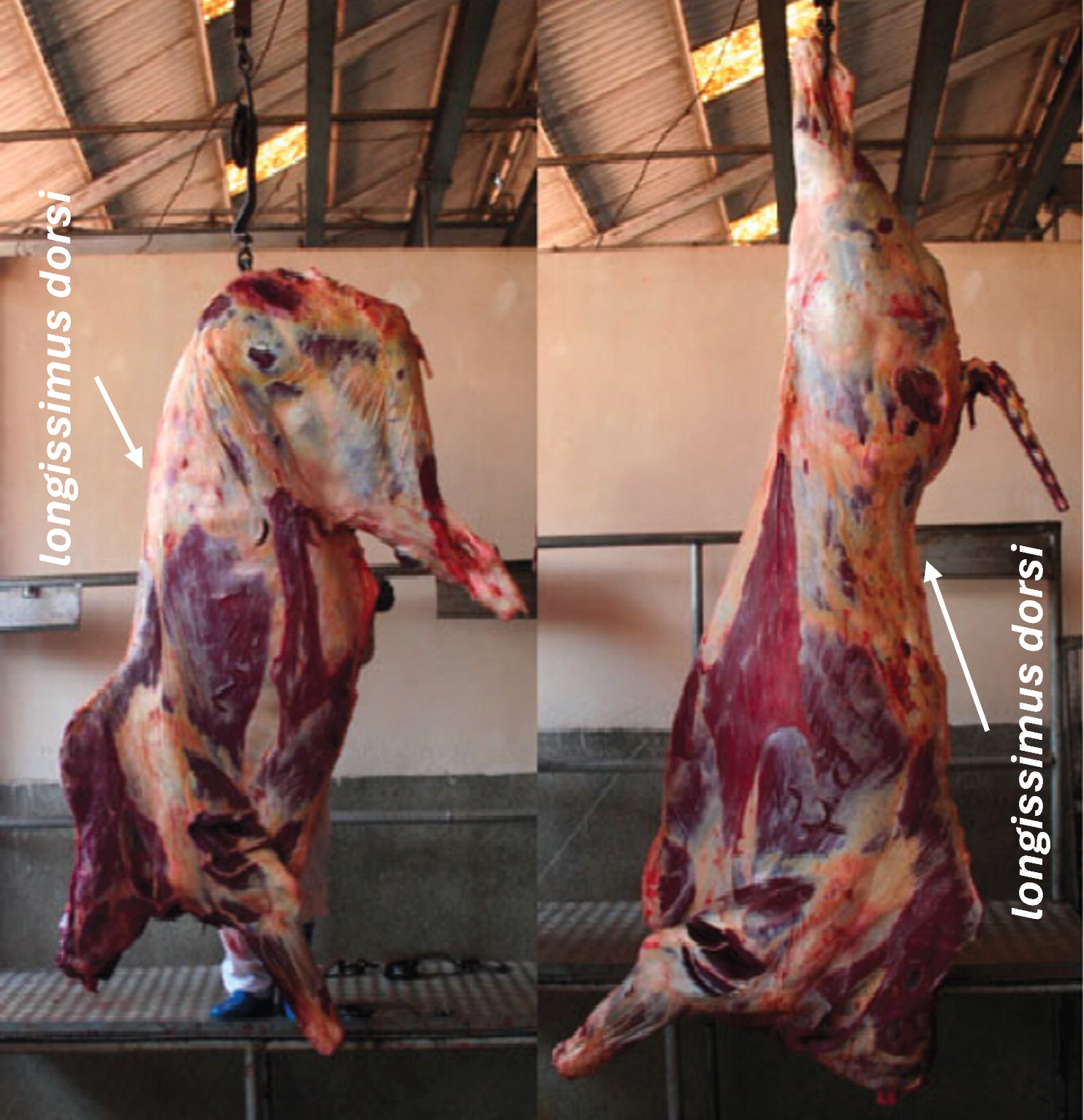 ![Left: Pelvic suspension. Right: Achilles suspension.](carcass.png){#fig-carcass} </div> In the @tbl-carcass-results are shown the average results from each cell in the design. | Suspension | Age 2y | Age 3y | Age 4y | |:------------|-------:|-------:|-------:| | Pelvic (A) | 58.5 | 65.0 | 66.0 | | Achilles (B)| 72.0 | 82.5 | 93.0 | : Mean values for the design (n = 15 in each group) {#tbl-carcass-results .hover .responsive} ::: {.callout-task} 1. Sketch these results with the response on the y-axis, one factor on the x-axis, and join the points based on the other factor. What is your first impression on the effect of age of the animal and of suspension method. * Further, does the lines seem to be deviating from being parallel? (This indicates interaction between the factors). 2. Write up a model including interaction term. 3. Write up the $H0$ (and the alternative) hypotheses for the main effects in this experiment. ::: | Source | SS | df | MS | F | p-value | |:---------------|--------:|---:|------:|--:|--------:| | Age | 3083.7 | | | | | | Suspension | 8410.0 | | | | | | Age*Suspension | | | | | | | Error | | | 375.0 | - | - | | Total | 43715.0 | 89 | - | - | - | : ANOVA table for response `shear force`. {#tbl-shear-force .hover .responsive} ::: {.callout-task} 4. Fill the missing values in the @tbl-shear-force. 5. What factors are having a significant effect (significance level of 0.05)? 6. Modify the two-way ANOVA model. Should the interaction be included in the final model for the present study? Why/Why not? 7. Toughness is explained by muscle fibers and connective tissue. The contribution from muscle fibers is impacted by suspension method. The contribution from connective tissue is impacted by age. Would you expect an effect of the interaction term between suspension method and age? Why/Why not? How does your answer correspond with the answers in question 6? 8. Traditionally, carcasses suspension is done by Achilles, what would you recommend based on this study? What are the limitations/assumptions for such a recommendation? * Hint: Have we checked all muscles? Look at the picture - do you think the conclusions extrapolate to other parts of the animal? ::: :::  ::: {#ex-stability-of-oil-2}  ::: ::: {.callout-exercise} ### Stability of oil under different conditions This exercise is a direct extension of @ex-stability-of-oil-under-different-conditions. Oil are primary made up of triglycerides, where some of the fatty acids are unsaturated. This causes such a product to be susceptible to oxidation both from chemical oxidative agents such as metal ions, or from exposure to light. Oxidation of the unsaturated fatty acids changes the sensorical and physical properties of the oil. In the southern part of Africa grows a robust bean - the Marama bean. This bean has a favorable dietary composition, including dietary fibers, fats and proteins, as most similar types of nuts, therefore this crop could be utilized for making healthy products by the locals for the locals. One such product is Marama bean oil. A study has been conducted to investigate the oxidative stability of the oil under various conditions. In the dataset `MaramaBeanOilOx.xlsx` are listed the results from such an experiment (including data from both normal and roasted beans). The experimental factors are: * Storage time (`Month`) * Product type (`Product`) * Storage temperature (`Temperature`) * Storage condition (`Light`) * Packaging air (`Air`) The response variable reflecting oxidative stability is peroxide value and named `PV`. The first three questions are identical to @ex-stability-of-oil-under-different-conditions. ::: {.callout-task} 1. Read in the data, and subset so that you only include data related to product type `Oil`. 2. Make descriptive plots of the response variable `PV` imposing storage temperature, condition, and time. * Hint: `factor(Temperature):Light` specifies all combinations of these two factors. `facet_grid(.~Month)` splits the plot into several plots according to Month. 3. What do you observe in terms of storage time, temperature and condition from this plot? 4. Based on the plot, suggest a model including the three factors `Month`, `Temperature` and `Light`. Which factors do you think is additive (i.e. have the same effect regardless of the other factors), and which do you think interacts? 5. Build a model including all combinations of the three factors. * That is: `m <- aov(data=Marama.oil, PV~factor(Temperature)*Light*factor(Month))`. 6. Check the assumption concerning the distribution of the residuals. If necessary, make an appropriate transformation of the response variable, and check that it is doing better in terms of distributional assumptions for the model residuals. 7. It seems like we need all combinations of everything. Construct a single variable, that has the seven levels indicating the design, and use this in an ANOVA model. * Hint: `Allcomp <- factor(Marama.oil$Temperature):Marama.oil$Light:factor(Marama.oil$Month` 8. Use `TukeyHSD()` on that model to make all pairwise comparisons of the seven individual levels. And comment on what you obtain. Does the initial plot correspond to the pairwise observations? ::: :::

Source	SSQ	DF	MS	\(F_{obs}\)	\(Pr(F_{df_A,df_e}>F_{obs})\)
Factor(A)	\(SS_A\)	\(df_A = k-1\)	\(MS_A = SS_A/df_A\)	\(F_A = MS_A/MS_e\)	\(p_A\)
Residuals	\(SS_e\)	\(df_e = n-k\)	\(MS_e = SS_e/df_e\)
Total	\(SS_{tot}\)	\(df_{tot} = n-1\)

Source	SSQ	DF	MS	\(F_{obs}\)	\(Pr(F_{df_{Source},df_e}>F_{obs})\)
Factor(A)	\(SS_A\)	\(df_A = k_A-1\)	\(MS_A = SS_A/df_A\)	\(F_A = MS_A/MS_e\)	\(p_A\)
Factor(B)	\(SS_B\)	\(df_B = k_B-1\)	\(MS_B = SS_B/df_B\)	\(F_B = MS_B/MS_e\)	\(p_B\)
Residuals	\(SS_e\)	\(df_e = n-df_A - df_B - 1\)	\(MS_e = SS_e/df_e\)
Total	\(SS_{tot}\)	\(df_{tot} = n-1\)

Source	SSQ	DF	MS	\(F_{obs}\)	\(Pr(F_{df_{Source},df_e}>F_{obs})\)
Factor(A)	\(SS_A\)	\(df_A = k_A-1\)	\(MS_A = SS_A/df_A\)	\(F_A = MS_A/MS_e\)	\(p_A\)
Factor(B)	\(SS_B\)	\(df_B = k_B-1\)	\(MS_B = SS_B/df_B\)	\(F_B = MS_B/MS_e\)	\(p_B\)
Factor(A*B)	\(SS_{AB}\)	\(df_{AB} = (k_A-1)(k_B-1)\)	\(MS_{AB} = SS_{AB}/df_{AB}\)	\(F_{AB} = MS_{AB}/MS_e\)	\(p_{AB}\)
Residuals	\(SS_e\)	\(df_e = n-df_A - df_B - df_{AB} - 1 = n - (k_A)(k_B)\)	\(MS_e = SS_e/df_e\)
Total	\(SS_{tot}\)	\(df_{tot} = n-1\)