Understand the different ingredients in the t-test.
Being able to calculate a t-test based on knowledge on sample means, standard deviations and number of observations.
Be able to compute a t-test for two samples with equal and unequal variance.
Understand the relation between confidence intervals for differences and a t-test for comparison of two means.
Comprehend that the generic procedure of a null-hypothesis tests is based on some measure of distance to the null-assumption and some relevant distribution to look-up that distance.
The research question goes on the difference between the two samples. Such as question is formalized statistically using the parameters of the two models under investigation and called a hypothesis. Further, a question of is formalized as the opposite; similarity.
That is the null hypothesis of no difference between the two sample means is formalized as:
\[
H0: \mu_1 = \mu_2
\]
If this hypothesis turns out not to be true. That is; there is a difference between the two distribution means, then this is referred to as the alternative hypothesis:
The standard deviation used here (\(s_{X_{pooled}}\)) is based on weighted average of the individual sample variances.
Example 10.1
Example 10.1 - Effect of caffeine on activity - hypothesis test
In Example 8.1 concerning the relation between caffeine and voluntary activity of mice, the running activity of mice in a wheel is recorded. In this example we wish to compare the mean activity of the two groups with either water- or Red bull as caffeine source in control runner female mice, and give a confidence interval for these means.
As such, from Example 8.3 the activity seems higher in the Red Bull treated group. The question we wish to answer is: Is there a difference between the two population means. In statistical terms this question is formalized as a hypothesis.
Note, that the spread \((\sigma)\) is assumed to be similar in the two groups.
Hypothesis
If we are interested in a difference, then we formulate the opposite, that is; the two population means are equal.
\[
H0: \mu_1 = \mu_2
\]
If this turns out not to be true, then the alternative is suggested to be:
\[
HA: \mu_1 \neq \mu_2
\]
A statistical test done via first constructing a measure of how far from the \(H0\) the data is. This is referred to as the test-statistic and then secondly this measure is translated in to a probability.
Test statistic \(H0\) sets the two means to be equal, so naturally a measure of how well this fits with data is reflected as the difference between the observed averages:
\[
\bar{X}_1 - \bar{X}_2
\]
where a large (positive or negative) value indicates descrepancy from \(H0\).
This distance depends on the scale of the data, why some kind of normalization needs to be encountered. Further, the number of samples used to calculate the means should also weight in. In total this leads to the t-test statistic.
We see that almost all the ingredients for calculating this is given via the descriptive statistics. The only thing needed is the pooled standard deviation (\(s_{pooled}\)), which is simply a weighted mean of the variances.
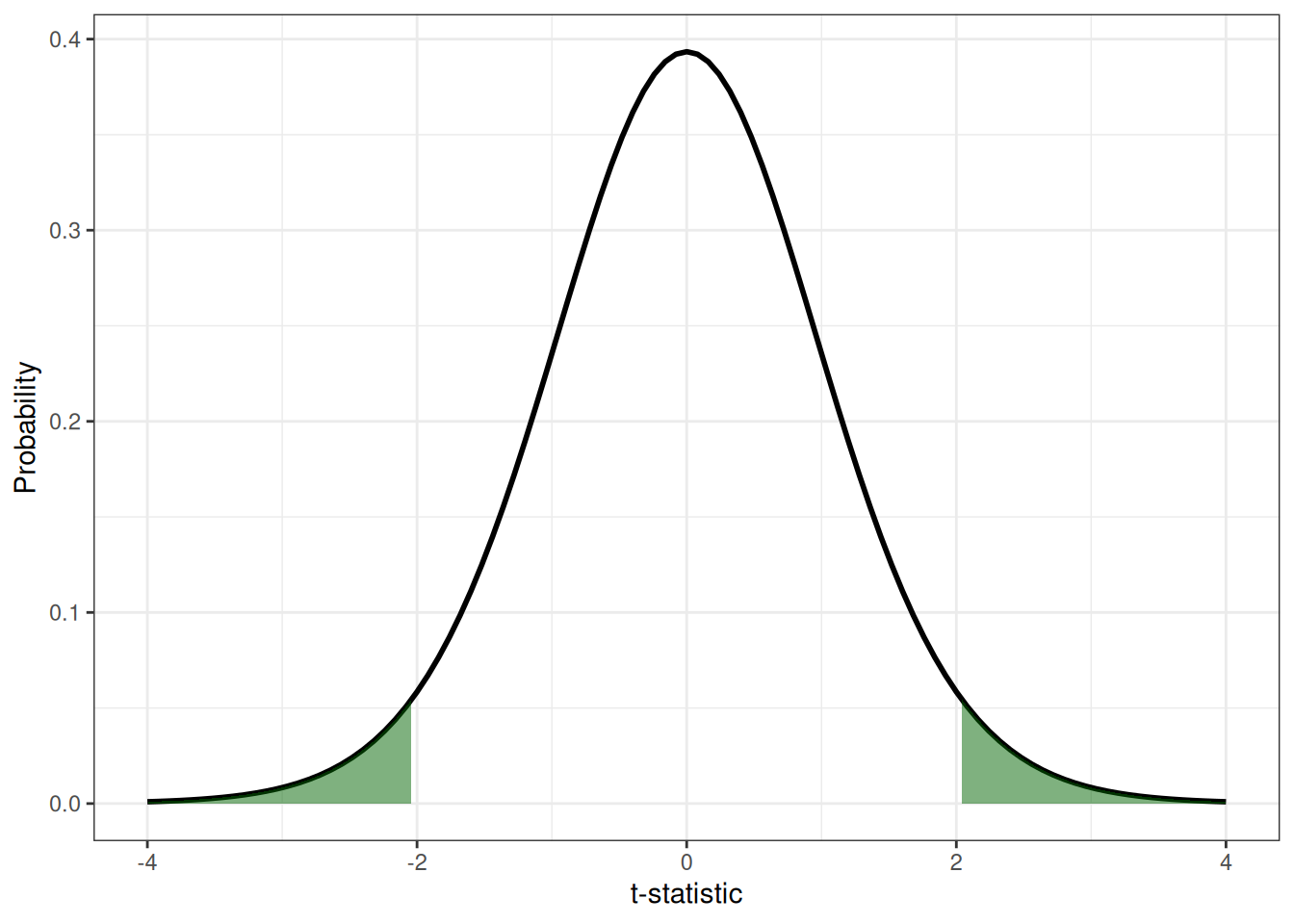
which corresponds to the colored areas shown in figure 10.1.
Code
# Dummy data to make geom_area actually plotdf <-data.frame(x =1, y =42)# Arguments for pt functiondtArgs <-list(df =20-2)# Critical valueslwrCrit <-qt(0.05/2, 30)uprCrit <-qt(1-0.05/2, 30)# Plotggplot(df, aes(x, y)) +xlim(-4, 4) +geom_function(fun = dt, args = dtArgs, linewidth =1 ) +geom_area(stat ="function", fun = dt, args = dtArgs, # Lower crit regionxlim =c(-5, lwrCrit), fill ="darkgreen", alpha =.5 ) +geom_area(stat ="function", fun = dt, args = dtArgs, # Upper crit regionxlim =c(uprCrit, 5), fill ="darkgreen", alpha =.5 ) +labs(x ="t-statistic",y ="Probability" ) +theme_bw()
Figure 10.1: The critical regions of the t-statistic for a t-test with \(\alpha = 0.05\) (i.e. the total area of the shaded areas is equal to \(0.05\)) and \(df = 20 - 2\).
This has no analytical solution, but can be assessed from tables or via pt() in R:
t_obs <-1.610df <-20-22* (1-pt(t_obs, df))
[1] 0.1247948
In conclusion; Although a difference in activity is observed when mice are given Red Bull compared to water, it is Not unlikely (\(p = 0.12\)) that this could be due to chance. Actually this would happen one out of eight times.
    Two Sample t-test

data:  x_subset[x_subset$Caffeine == "Water", "RPM7"] and x_subset[x_subset$Caffeine == "Red Bull", "RPM7"]
t = -1.615, df = 18, p-value = 0.1237
alternative hypothesis: true difference in means is not equal to 0
95 percent confidence interval:
 -3.5208153  0.4604011
sample estimates:
mean of x mean of y
 8.649382 10.179589
10.3 Paired T-test - in short
A special case, is where the two samples (\(X_{11},X_{12},X_{13},...,X_{1n}\) and \(X_{21},X_{22},X_{23},...,X_{2n}\)) are paired. That is for example measurements before and after treatment on the same set of samples or when the same assessor in a sensorical panel scores two different product types.
The question of interest is still the same; namely is there a difference between the two populations, however, the statistics is slightly different.
10.3.1 Model
The model of the data is extended with a sequence of differences
Where \(D_i\) is the difference between the responses for each of the paired observations \(i\) (\(i = 1,2,\ldots,n\)), and \(s_D\) is the observed standard deviation calculated on \(D_1,D_2,\ldots,D_n\).
10.3.2 Hypothesis
The hypothesis of similarity is then formalized on \(\mu_D\):
Which is translated to a p-value through a \(\mathcal{T}_{df}\) with \(df = n-1\) degrees of freedom.
As such, the test statistics only sees the original data via paired differences, and hence become a specialty of the single-sample case.
Example 10.2
Example 10.2 - Natural phenolic antioxidants for meat preservation - paired T-test
This example is based on the sensory data on the meat sausages treated with green tea (GT) and rosemary extract (RE) or control, used previously in Example 6.1
T-tests can be used to evaluate the effects (the response of a single variable) of two treatments against each other. Here, we use the week 4 data, and compare the rosemary extract treatment to the control.
Plot data
First the data under investigation is plotted - only week 4, control, and RE samples are used (figure 10.2).
# Subset data such that Treatment = "Control" or "RE" AND week = 4 df <- X[X$Treatment %in%c("Control", "RE") & X$week ==4, ]ggplot(df, aes(Treatment, Texture_Boiled_egg_white, group = Assessor)) +geom_point() +geom_line() +theme_bw()
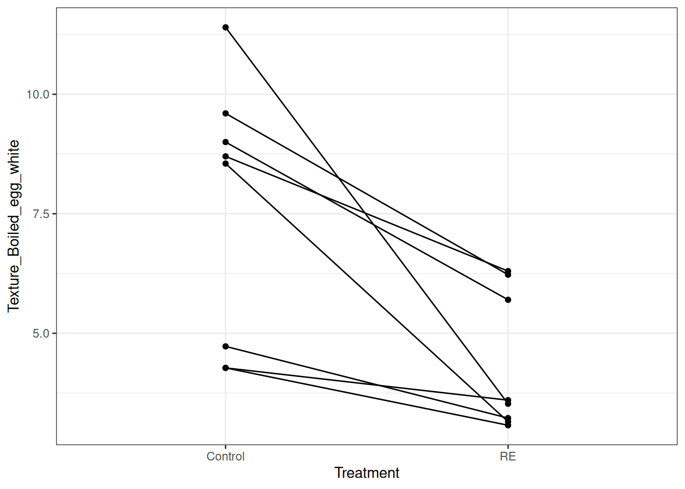
Figure 10.2: Paired sets of data points for the boiled egg texture variable in week 4 of the experiment. Each line represents a single assessor scoring both samples.
The figure clearly shows that there is huge variation related to Assessor (connected by lines). Although the distributions of the two groups are overlapping, ALL assessors scores the RE sample lower than the Control sample.
Define subsets of data
# Subset data such that Treatment = "Control" AND week = 4controlWeek4 <- X[X$Treatment =="Control"& X$week ==4, ]# Subset data such that Treatment = "RE" AND week = 4REWeek4 <- X[X$Treatment =="RE"& X$week ==4, ]
Be aware that the Assessors are ordered ensuring pairing in the two arrays controlWeek4 and REWeek4. Take precaution, as this might not always be the case!
Model of data
As it is the same assesors that are used for evaluation of both products the model of the data becomes:
where \(D_i\) is the difference between rosemary extract- and control treated sausages with respect to the sensorical score (texture - boiled egg) for assessor \(i\) (\(i = 1,2,\ldots,n\))
*Hypothesis
If we are interested in a difference, then we formulate the opposite, that is; on average the difference between sensorical scores are \(0\).
\[\begin{equation}
H0: \mu_D = 0
\end{equation}\]
If this turns out not to be true, then the alternative is suggested to be:
T-test on the boiled egg texture variable
The T-test should be a paired T-test, since it is the same assosors tasting each of the treated sausages.
t.test(controlWeek4$Texture_Boiled_egg_white, REWeek4$Texture_Boiled_egg_white,paired = T )
    Paired t-test

data:  controlWeek4$Texture_Boiled_egg_white and REWeek4$Texture_Boiled_egg_white
t = 3.7747, df = 7, p-value = 0.00694
alternative hypothesis: true mean difference is not equal to 0
95 percent confidence interval:
 1.20123 5.23002
sample estimates:
mean difference
       3.215625
The p-value is \(p = 0.007\) and the null-hypothosis must therefore be rejected meaning there is a very significant difference in boiled egg texture between the control and rosemary extracted treated samples.
T-test on the salty taste variable
In a similar fashion another sensorical variable is tested; namely salty taste.
t.test(controlWeek4$Taste_Salty, REWeek4$Taste_Salty,paired = T )
    Paired t-test

data:  controlWeek4$Taste_Salty and REWeek4$Taste_Salty
t = 0.98163, df = 7, p-value = 0.359
alternative hypothesis: true mean difference is not equal to 0
95 percent confidence interval:
 -0.5811623  1.4061623
sample estimates:
mean difference
         0.4125
The p-value is \(p = 0.36\) and the null-hypothosis can therefore not be rejeceted, meaning there is no significant difference in salty taste between the control and rosemary extract treated samples.
Comparison with PCA results
When the results obtained from the T-tests are compared to a PCA on the week 4 data, it can be seen that they are in agreement. The very significant effect of the rosemary extract treatment on the boiled egg texture corresponds well with the loading being strongly associated with the control samples, in a direction which seems to be explanatory for the difference between the roseary extract- and control treatment groups. The non-significant effect on the salty taste variable is congruent with its loading being located in a direction which does not seem to be of importance in the separation of the control and treated groups.
10.4 Videos
10.4.1 Hypothesis Testing and The Null Hypothesis, Clearly Explained - StatQuest
10.4.2 p-values: What they are and how to interpret them - StatQuest
10.4.3 Test Statistics - CrashCourse
10.4.4 T-Tests: A Matched Pair Made in Heaven - CrashCourse
10.5 Exercises
Exercise 10.1
Exercise 10.1 - T-test
T-test comparison of a womens football team and a mens football team. The mean weight of the mens team is \(\bar{X}_{men} = 82kg\) with a standard deviation of \(s_{men} = 8kg\), while the womens team has a mean weight of \(\bar{X}_{women} = 61kg\) and a standarddeviation of \(s_{women} = 6kg\). There are 11 players on each team.
Tasks
State the model and hypothesis
Calculate the test statistic (\(t_{obs}\))
Calculate the p-value
Exercise 10.2
Exercise 10.2 - Diet and fat metabolism - T-test by hand
The diet is a central factor involved in general health, and especially in relation to obesity, where a balance between intake of protein, fat and carbohydrates, as well as type of these nutrients seems important. Therefor various controlled studies are conducted to show the effect of different diets. A study examining the effect of protein from milk (casein or whey) and amount of fat on growth biomarkers of fat metabolism and type I diabetes was conducted in \(40\) mouse over an intervention period of \(14\) weeks.
For this exercise we are going to focus on cholesterol as a biomarker related to fat metabolism, and on a low fat diet (LF) and a high fat diet (HF). The cholesterol level at the end of the \(14\) week intervention is listed below (table 10.1).
Table 10.1: Cholesterol samples from the end of week 14 for the low-fat (LF) and high-fat (HF) diet.
Diet
\(\sum X\)
\(\sum X^2\)
LF
3.97
3.69
2.61
4.03
2.98
3.51
3.62
2.81
3.62
3.53
34.37
120.20
HF
4.68
3.60
4.84
4.92
3.70
4.83
3.38
4.62
4.60
4.84
4.84
4.54
5.27
4.26
4.3
67.29
305.92
This exercise is supposed to be done by hand where the computer only is used as a pocket calculator.
Tasks
Calculate descriptive statistics for these data.
Sketch these results in a graph (by pen and paper - no computer)
Give a frank guess on cholesterol differences between diets.
State a hypothesis, and calculate the test statistics and the corresponding p-value.
What assumptions did you make concerning the variances in the two distributions? What alternatives do you have?
Give a confidence interval for the difference between diets.
How does the t-test result (p-value) correspond to the confidence interval?
Exercise 10.3
Exercise 10.3 - Diet and fat metabolism - T-test in R
This exercise repeats some of the elements from Exercise 10.2 using R including an extension of the panel of relevant biomarkers and utilization of PCA to get a comprehensive overview.
The data can be found in the file Mouse_diet_intervention.xlsx. The code below imports the data, and subsets on two (of the three diets). The factor diet is called diet_fat, whereas cholesterol is called cholesterol.
Tasks
Repeat the analysis of Exercise 10.2 using R, including plotting and testing.
Hint: For testing you might want to predefine the response and factor and then use the function t.test() to run the analysis, which actually returns most of the relevant results - see the code box below.
How robust are the results towards transformation of the response or extreme samples?
In addition to cholesterol, other biomarkers have been measured, such as insuline, triglycerides etc.
Tasks
Use one of these additional biomarkers as measure of health status, and repeat the analysis comparing dietary fat (including plotting).
Make a PCA on the biomarkers insulin, cholesterol, triglycerides, NEFA, glucose, and HbA1c, and plot the results.
NEFA = nonesterified fatty acids.
Comment on the results. Do the T-test results fit with the PCA results? Are there other markers of dietary fat intake? Does the correlation structure make sense? (The later is hard to answer without physiological knowledge, but give it a shot)
# Import datamouse <-read_excel("Mouse_diet_intervention.xlsx")# Include only rows where diet_protein = caseinmouse <- mouse[mouse$diet_protein =="casein", ]# Predefine response and factordiet <- mouse$diet_faty <- mouse$cholesterol
Exercise 10.4
Exercise 10.4 - Fiber and cholesterol
Fiber is suspected to have benificial physiological activity if being a part of a regular diet. In this study \(n = 13\) healthy young men and women were enroled in a trial to unravel the effect of fiber supplement. At baseline (that is before dietary intervention), the persons were screned for a range of biomarkers in the blood including cholesterol fractions. Then, they were put on a diet with supplementation of dietary fibers for a period of \(30\) days. In the dataset FiberData.xlsx, the baseline levels (_t0), and end of trial levels (_t30) are listed for total-, hdl- and ldl cholesterol. The data is a part of a larger study conducted at Department of Nutrition Exercise and Sports.
Tasks
Analyse if there is an effect of the fiber intervention on these biomarkers. That includes; inspection of raw data, possible transformations, visulization of effects, descriptive statistics, test of effect and presentation of relevant confidence intervals.
Exercise 10.5
Exercise 10.5 - Stability of oil under different conditions
Oil are primary made up of triglycerides, where some of the fatty acids are unsaturated. This causes such a product to be susceptible to oxidation both from chemical oxidative agents such as metal ions, or from exposure to light. Oxidation of the unsaturated fatty acids changes the sensorical and physical properties of the oil.
In the southern part of Africa grows a robust bean - the Marama bean. This bean has a favorable dietary composition, including dietary fibers, fats and proteins, as most similar types of nuts, therefor this crop could be utilized for making healthy products by the locals for the locals. One such product is Marama bean oil. A study has been conducted to investigate the oxidative stability of the oil under various conditions. In the dataset MaramaBeanOilOx.xlsx are listed the results from such an experiment (including data from both normal and roasted beans). The experimental factors are:
Storage time (Month)
Product type (Product)
Storage temperature (Temperature)
Storage condition (Light)
Packaging air (Air)
And the response variable reflecting oxidative stability is peroxide value and named PV.
Tasks
Read in the data, and subset so that you only include data related to product type Oil.
Make descriptive plots of the response variable PV imposing storage-temperature, condition and time.
Hint: factor(Temperature):Light specifies all combinations of these two factors. facet_grid(.~Month) splits the plot into several plots according to Month.
What do you observe in terms of storage- time, temperature and condition from this plot?
Some of the differences is so pronounced that testing seems irrelevant. However, there are small differences between storage temperature at storage condition dark.
Zack out the data for these two groups at storage time = 0.5 month, and make a comparison.
Do the same at storage time = 1 month.
We would like to generate profiles for each condition over time, reflecting centrality and dispersion. In order to get there, we need to massage the data a little. The function summarySE() from the package Rmisc is a nice tool to construct a dataset with summary statistics. Try to run the code below - what have we learned about oil oxidation from this study?
# Compute summary table for "PV"maramaSummary <-summarySE(maramaOil, measurevar ="PV",groupvars =c("Light", "Temperature", "Month"))# Repeat time = 0 for all conditionsM1 <- maramaSummary[1, ]M1$Light <-"light"M1$Temperature <-25M2 <- maramaSummary[1, ]M2$Temperature <-35Mtot <-rbind(maramaSummary, M1, M2)# Plot a nice oxidation graph with errorbarsggplot(Mtot, aes(x = Month, y = PV, color =factor(Temperature):Light)) +geom_point() +geom_line() +geom_errorbar(aes(ymin = PV - se, ymax = PV + se), width = .03) +theme_bw()
Exercise 10.6
Exercise 10.6 - Aroma in milk and cheese
In order to increase the biodiversity of hayfields it is of interest growing different kinds of herbs together with the hay. Hay is used for feeding of cows. Type of feed may affect the amount and type of flavor components in the milk as well as the flavor components in cheese made from the milk. Hence, increasing the biodiversity of hayfields used for cow feed may impact the taste of milk and cheese. An experiment was conducted in order to investigate this. In the experiment cows were fed three different diets:
Feed 1: Ryegrass and white clover
Feed 2: Feed 1 + red clover, chicory and ribwort plantain
Flavor components were quantified in the raw milk as well as in the cheese after \(12\) months of ripening. Three farmers (G, H, and P) participated in the experiment. Furthermore, controls (K), consisting of bulk milk samples from the dairy, are included. The data are found in the file Milk_Cheese_Aroma.xlsx.
Data are originating from the EcoServe project and is kindly provided by Thomas Bæk Pedersen, Department of Food Science, University of Copenhagen.
Tasks
Import the data set.
Open the data and get familiar with the data set (that could include something like; how many samples, how many samples from each combination of feed and farmer, how many variables, and some descriptive plots of some of them).
In this exercise we are interested in making a pairwise comparison to investigate whether differences exists between the feedings. Hence, for now we will exclude the controls.
Tasks
Make two subsets of the data; one subset for milk samples and one subset for cheese samples. Exclude controls in the subsets.
Investigate a given aroma compound (e.g. Limonene) in the milk subset. This can be done by e.g. making a boxplot with feed on the x-axis and filling color according to farmer. Do you see any systematic effect of feed?
# Investigate the code and create the two subsets (one for cheese and one for milk).# What does the "&", "|", and "!" do?Milk <-subset(Data, Sample =="Milk"& Farmer =="K")Milk <-subset(Data, Sample =="Milk"&!Farmer =="K")Milk <-subset(Data, Sample =="Milk"| Farmer =="K")Milk <-subset(Data, Sample =="Milk"|!Farmer =="K")# Make a boxplotggplot(yourDataHere, aes(xVariable, yVariable, fill = yourFactor)) +geom_boxplot()
In a paired t-test we will investigate whether there is a difference between feed 1 and feed 3. In a paired t-test we are investigating if the mean of differences between pairs is significantly different from zero. The following steps will take you through the test.
Tasks
Calculate the difference (for e.g. Limonene) between each pair. Note that these differences now represent your sample
feed1 <-subset(Milk, Feed =="I") # Extract feed Ifeed1 <- feed1[with(feed1, order(Farmer)), ] # Sort according to farmerfeed3 <-subset(Milk, Feed =="III") # Extract feed IIIfeed3 <- feed3[with(feed3, order(Farmer)), ] # Sort according to farmerdiff <- feed1 - feed3 # Compute the difference
Tasks
Make a boxplot of the differences.
Add to the boxplot a zero line and the mean of the differences
Discuss the plot
Why do we add a line with intercept y=0? Why do we add the mean?
feed1 <-subset(Milk, Feed =="I") # Extract feed Ifeed1 <- feed1[with(feed1, order(Farmer)), ] # Sort according to farmerfeed3 <-subset(Milk, Feed =="III") # Extract feed IIIfeed3 <- feed3[with(feed3, order(Farmer)), ] # Sort according to farmerdiff <-data.frame("diff"= feed1$Limonene - feed3$Limonene) # Compute the differencemeanDiff <-mean(diff$diff) # Calculate mean of differenceggplot(diff, aes(x =1, y = diff)) +geom_boxplot() +geom_hline(aes(yintercept =0), color ="red", linetype ="dotted") +geom_point(x =1, y = meanDiff, color ="darkred", size =5)
We have now calculated the differences and we have calculated the mean of the differences. However, the mean is an estimated value and in order to find out whether there is a significant difference between feed 1 and feed 3, we need to calculate the confidence interval round the mean.
Tasks
Calculate the mean and the standard deviation of the differences and use these calculations to find the confidence interval of the mean.
For a 95% confidence interval you can find the critical t-value by calling abs(qt(0.025,df)) for a two sided test. How would the R-call look if you were calculating the critical t-value for a one-sided test?
Is zero included in the confidence interval? What does this mean?
Calculate the t-statistic. Is there a significant difference between the two feedings?
Understand the following code and call it in R.
Understand the output and compare the confidence interval and the t-statistics with what you calculated in question 6 and question 7.
t.test(feed1$Limonene, feed3$Limonene,mu =0, alt ='two.sided', paired = T, conf.level =0.95)
Now investigate the cheese-subset. Pick the same aroma compound you were working on during the milk-subset. Do you think there is a difference in the aroma compound between feed I and feed III when looking at the cheese-samples? Write the hypothesis and test it using a paired t-test.
Use the R-call t.test(……).
If you were a farmer, would you be worried that increasing the biodiversity of your hayfields with herbs would result in altered taste in the milk/cheese?
Exercise 10.7
Exercise 10.7 - Power of paired tests
In Exercise 10.4Fiber and Cholesterol you have probably used either a paired t-test or a two-sample t-test. Try to conduct both of these tests and see the difference. What needs to be full filled in order to make a paired test? How many participants would have been enrolled in the study, in the case where a two sample t-test were used for inferential analysis of the data?
Exercise 10.8
Exercise 10.8 - Confidence intervals
The datafile Wine.xlsx lists aroma compounds from different wines from four countries. The compound Acetic acid has a skewed distribution, and therefore needs an appropriate transformation. Calculate the center of the distribution for each country and give a confidence interval for this parameter, where you take into account the need for transformation, but still want to report the results in original units.
The R function t.test() is capable of doing some of the calculations.
Source Code
# T-test```{r}#| label: t-test-setup#| echo: false#| message: false#| warning: falselibrary(ggplot2)library(here)library(dplyr)load(here("data", "MouseWheelCaffeine.RData"))x_subset <- X |>filter( MouseType =="Control runner", gender =="Female", Caffeine %in%c("Red Bull", "Water") )```::: {.callout-tip}## Learning objectives* Understand the different ingredients in the t-test. * Being able to calculate a t-test based on knowledge on sample means, standard deviations and number of observations. * Be able to compute a t-test for two samples with equal and unequal variance. * Understand the relation between confidence intervals for differences and a t-test for comparison of two means. * Comprehend that the generic procedure of a null-hypothesis tests is based on some measure of distance to the null-assumption and some relevant distribution to look-up that distance. :::## Reading material * [Independent T-test - in short](#sec-independent-t-test)* [Paired T-test - in short](#sec-paired-t-test)* Videos on the elements of statistical testing focusing on hypothesis testing: * [Hypothesis Testing and The Null Hypothesis, Clearly Explained](#sec-nhst-statquest) * [p-values: What they are and how to interpret them](#sec-p-values-statquest)* Videos on the test statistics and the T-test: * [Test Statistics](#sec-test-statistics-crashcourse) * [T-Tests: A Matched Pair Made in Heaven](#sec-t-test-crashcourse)* Chapter 3 of [*Introduction to Statistics*](https://02402.compute.dtu.dk/enotes/book-IntroStatistics) by Brockhoff## Independent T-test - in short {#sec-independent-t-test}### Models of two samples First of all the data are characterized by two models, here normally distributed samples: $$X_{11},X_{12},X_{13},...,X_{1n_1} \sim \mathcal{N}(\mu_1,\sigma_1^2)$$$$X_{21},X_{22},X_{23},...,X_{2n_2} \sim \mathcal{N}(\mu_2,\sigma_2^2)$$### HypothesisThe research question goes on the difference between the two samples. Such as question is formalized statistically using the parameters of the two models under investigation and called a hypothesis. Further, a question of \textit{difference} is formalized as the opposite; similarity.That is the null hypothesis of no difference between the two sample means is formalized as: $$H0: \mu_1 = \mu_2$$If this hypothesis turns out *not* to be true. That is; there is a difference between the two distribution means, then this is referred to as the alternative hypothesis: $$HA: \mu_1 \neq \mu_2$$or directional: $$H_A: \mu_1>\mu_2 \ \ \ or \ \ \ H_A: \mu_1<\mu_2$$$$H_A: \mu_1<\mu_2$$### Test statisticFrom these data, a t-statistic $t_{obs}$ can be calculated: $$t_{obs} = \frac{\bar{X_1} - \bar{X_2}}{s_{pooled}\sqrt{\frac{1}{n_1} + \frac{1}{n_2}}}$$where $s_{pooled}$ is the pooled standard deviation, which is simply a weighted mean of the variances.$$s_{pooled}^2 = \frac{(n_1 - 1)s_1^2 + (n_2-1)s_2^2}{n_1 + n_2-2}$$Alternatively, this formulation is equivalent: $$t_{obs} = \frac{\bar{X_1} - \bar{X_2}}{\sqrt{\frac{s_{X_1}^2}{n_1} + \frac{s_{X_2}^2}{n_2}}}$$### Test probabilityThis t-statistics for the non-directional two-sided test can be translated into a probability under the null hypothesis (of no difference).$$P = 2 \cdot P(T_{df} \geq |t_{obs}|) = 2 \cdot (1 - P(T_{df} \leq |t_{obs}|))$$Alternatively, one can calculate a confidence interval for the differences between the means, which leads to the same interpretation of the results:$$\bar{X_1} - \bar{X_2} \pm t_{1 - \alpha/2}s_{X_{pooled}}\sqrt{\frac{1}{n_1} + \frac{1}{n_2}}$$The standard deviation used here ($s_{X_{pooled}}$) is based on weighted average of the individual sample variances. ::: {#exa-effect-of-caffeine-hypothesis-test}<!-- Cross-ref anchor -->:::::: {.callout-example}### Effect of caffeine on activity - hypothesis testIn @exa-effect-of-caffeine concerning the relation between caffeine and voluntary activity of mice, the running activity of mice in a wheel is recorded. In this example we wish to compare the mean activity of the two groups with either water- or Red bull as caffeine source in control runner female mice, and give a confidence interval for these means.As such, from @exa-effect-of-caffeine-conf-int the activity seems higher in the Red Bull treated group. The question we wish to answer is: Is there a difference between the two population means. In statistical terms this question is formalized as a hypothesis.First, models for the data is suggested$$X_1 \sim \mathcal{N}(\mu_1,\sigma^2)$$$$X_2 \sim \mathcal{N}(\mu_2,\sigma^2) $$Note, that the spread $(\sigma)$ is assumed to be similar in the two groups.**Hypothesis** If we are interested in a difference, then we formulate the opposite, that is; the two population means are equal.$$H0: \mu_1 = \mu_2$$If this turns out *not* to be true, then the alternative is suggested to be:$$HA: \mu_1 \neq \mu_2$$A statistical test done via first constructing a measure of *how far* from the $H0$ the data is. This is referred to as the test-statistic and then secondly this measure is translated in to a probability.**Test statistic** $H0$ sets the two means to be equal, so naturally a measure of how well this fits with data is reflected as the *difference* between the observed averages: $$\bar{X}_1 - \bar{X}_2$$where a large (positive or negative) value indicates descrepancy from $H0$. This distance depends on the scale of the data, why some kind of normalization needs to be encountered. Further, the number of samples used to calculate the means should also weight in. In total this leads to the t-test statistic.$$t_{obs} = \frac{\bar{X}_1 -\bar{X}_2}{s_{pooled} \sqrt{\frac{1}{n_1} + \frac{1}{n_2}}}$$We see that almost all the ingredients for calculating this is given via the descriptive statistics. The only thing needed is the pooled standard deviation ($s_{pooled}$), which is simply a weighted mean of the variances.\begin{align}s_{pooled}^2 &= \frac{(n_1 - 1)s_1^2 + (n_2-1)s_2^2}{n_1 + n_2-2} \\&= \frac{(11 - 1) \cdot 2.1^2 + (9-1)\cdot 2.1^2}{11 + 9-2} \\&= 2.1^2 \end{align}This leads to:\begin{align}t_{obs} &= \frac{\bar{X}_1 -\bar{X}_2}{s_{pooled} \sqrt{\frac{1}{n_1} + \frac{1}{n_2}}} \\&= \frac{8.6 -10.2}{2.1 \sqrt{\frac{1}{11} + \frac{1}{9}}} \\&= 1.61 \end{align}**P-value** The test statistics is translated to a probability by the following:$$P = 2 \cdot P(T_{df} \geq |t_{obs}|) = 2 \cdot (1 - P(T_{df} \leq |t_{obs}|))$$which corresponds to the colored areas shown in @fig-critical-regions-t-dist.```{r}#| label: fig-critical-regions-t-dist#| fig-cap: The critical regions of the t-statistic for a t-test with $\alpha = 0.05$ (i.e. the total area of the shaded areas is equal to $0.05$) and $df = 20 - 2$.#| code-fold: true# Dummy data to make geom_area actually plotdf <-data.frame(x =1, y =42)# Arguments for pt functiondtArgs <-list(df =20-2)# Critical valueslwrCrit <-qt(0.05/2, 30)uprCrit <-qt(1-0.05/2, 30)# Plotggplot(df, aes(x, y)) +xlim(-4, 4) +geom_function(fun = dt, args = dtArgs, linewidth =1 ) +geom_area(stat ="function", fun = dt, args = dtArgs, # Lower crit regionxlim =c(-5, lwrCrit), fill ="darkgreen", alpha =.5 ) +geom_area(stat ="function", fun = dt, args = dtArgs, # Upper crit regionxlim =c(uprCrit, 5), fill ="darkgreen", alpha =.5 ) +labs(x ="t-statistic",y ="Probability" ) +theme_bw()```This has no analytical solution, but can be assessed from tables or via `pt()` in R:```{r}t_obs <-1.610df <-20-22* (1-pt(t_obs, df))```In conclusion; Although a difference in activity is observed when mice are given Red Bull compared to water, it is Not unlikely ($p = 0.12$) that this could be due to chance. Actually this would happen one out of eight times. The entire procedure can be done in R:```{r}t.test(x_subset[x_subset$Caffeine =="Water", "RPM7"], x_subset[x_subset$Caffeine =="Red Bull", "RPM7"],var.equal = T)```::: <!-- End example callout -->## Paired T-test - in short {#sec-paired-t-test}A special case, is where the two samples ($X_{11},X_{12},X_{13},...,X_{1n}$ and $X_{21},X_{22},X_{23},...,X_{2n}$) are paired. That is for example measurements before and after treatment on the same set of samples or when the same assessor in a sensorical panel scores two different product types.The question of interest is still the same; namely is there a difference between the two populations, however, the statistics is slightly different.### ModelThe model of the data is extended with a sequence of differences\begin{align} & D_1,D_2,\ldots,D_n \nonumber \\= & (X_{12} - X_{11}), (X_{22} - X_{21}), \ldots , (X_{n2} - X_{n1}) \\\sim & \mathcal{N}(\mu_{D},\sigma_{D}^2) \nonumber \end{align}Where $D_i$ is the difference between the responses for each of the paired observations $i$ ($i = 1,2,\ldots,n$), and $s_D$ is the observed standard deviation calculated on $D_1,D_2,\ldots,D_n$. ### HypothesisThe hypothesis of similarity is then formalized on $\mu_D$: \begin{equation}H0: \mu_D = 0\end{equation}Often with the alternative of a difference: \begin{equation}HA: \mu_D \neq 0\end{equation}### Test Statistic\begin{equation}t_{obs} = \frac{\bar{D} }{s_{D} / \sqrt{n}}\end{equation}Which is translated to a p-value through a $\mathcal{T}_{df}$ with $df = n-1$ degrees of freedom. As such, the test statistics only sees the original data via paired differences, and hence become a specialty of the single-sample case. ::: {#exa-natural-phenolic-antiox-paired-t-test}<!-- Cross-ref anchor -->:::::: {.callout-example}### Natural phenolic antioxidants for meat preservation - paired T-test```{r}#| label: paired-t-test-example-setup#| echo: false#| message: false#| warning: falseload(here("data", "meat_data.RData"))```This example is based on the sensory data on the meat sausages treated with green tea (GT) and rosemary extract (RE) or control, used previously in @exa-phenolic-antiox-pcaT-tests can be used to evaluate the effects (the response of a single variable) of two treatments against each other. Here, we use the *week 4* data, and compare the rosemary extract treatment to the control.**Load the data and libraries** Remember to set your [working directory](#sec-r-basics-working-directory).```{r}#| eval: false#| code-line-numbers: falselibrary(ggplot2)load("meat_data.RData")```**Plot data** First the data under investigation is plotted - only *week 4*, *control*, and *RE* samples are used (@fig-paired-data-RE). ```{r}#| label: fig-paired-data-RE#| fig-cap: Paired sets of data points for the *boiled egg texture* variable in week 4 of the experiment. Each line represents a single assessor scoring both samples.# Subset data such that Treatment = "Control" or "RE" AND week = 4 df <- X[X$Treatment %in%c("Control", "RE") & X$week ==4, ]ggplot(df, aes(Treatment, Texture_Boiled_egg_white, group = Assessor)) +geom_point() +geom_line() +theme_bw()```The figure clearly shows that there is huge variation related to Assessor (connected by lines). Although the distributions of the two groups are overlapping, *ALL* assessors scores the *RE* sample lower than the *Control* sample. **Define subsets of data** ```{r}# Subset data such that Treatment = "Control" AND week = 4controlWeek4 <- X[X$Treatment =="Control"& X$week ==4, ]# Subset data such that Treatment = "RE" AND week = 4REWeek4 <- X[X$Treatment =="RE"& X$week ==4, ]```Be aware that the Assessors are ordered ensuring pairing in the two arrays `controlWeek4` and `REWeek4`. Take precaution, as this might not always be the case!**Model of data** As it is the *same* assesors that are used for evaluation of both products the model of the data becomes: \begin{equation}X_{control} \sim \mathcal{N}(\mu_{control},\sigma_{control}^2) \ \ \text{and} \ \ X_{RE} \sim \mathcal{N}(\mu_{RE},\sigma_{RE}^2)\end{equation}\begin{align}D_1,D_2,\ldots,D_n \sim \mathcal{N}(\mu_{D},\sigma_{D}^2)\end{align}where $D_i$ is the difference between rosemary extract- and control treated sausages with respect to the sensorical score (texture - boiled egg) for assessor $i$ ($i = 1,2,\ldots,n$)\begin{align}& D_1,D_2,\ldots,D_n = (X_{1,RE} - X_{1,control}), (X_{2,RE} - X_{2,control}), \ldots , (X_{n,RE} - X_{n,control}).\end{align}***Hypothesis** If we are interested in a difference, then we formulate the opposite, that is; on average the difference between sensorical scores are $0$. \begin{equation}H0: \mu_D = 0\end{equation}If this turns out *not* to be true, then the alternative is suggested to be:\begin{equation}HA: \mu_D \neq 0\end{equation}**T-test on the boiled egg texture variable** The T-test should be a paired T-test, since it is the same assosors tasting each of the treated sausages.```{r}t.test(controlWeek4$Texture_Boiled_egg_white, REWeek4$Texture_Boiled_egg_white,paired = T )```The p-value is $p = 0.007$ and the null-hypothosis must therefore be rejected meaning there is a very significant difference in boiled egg texture between the control and rosemary extracted treated samples.**T-test on the salty taste variable** In a similar fashion another sensorical variable is tested; namely *salty taste*.```{r}t.test(controlWeek4$Taste_Salty, REWeek4$Taste_Salty,paired = T )```The p-value is $p = 0.36$ and the null-hypothosis can therefore not be rejeceted, meaning there is no significant difference in salty taste between the control and rosemary extract treated samples.**Comparison with PCA results** When the results obtained from the T-tests are compared to a PCA on the *week 4* data, it can be seen that they are in agreement. The very significant effect of the rosemary extract treatment on the boiled egg texture corresponds well with the loading being strongly associated with the control samples, in a direction which seems to be explanatory for the difference between the roseary extract- and control treatment groups. The non-significant effect on the salty taste variable is congruent with its loading being located in a direction which does not seem to be of importance in the separation of the control and treated groups.:::<!-- End example callout -->## Videos### Hypothesis Testing and The Null Hypothesis, Clearly Explained - *StatQuest* {#sec-nhst-statquest}{{< video https://www.youtube.com/watch?v=0oc49DyA3hU >}}### p-values: What they are and how to interpret them - *StatQuest* {#sec-p-values-statquest}{{< video https://www.youtube.com/watch?v=vemZtEM63GY >}}### Test Statistics - *CrashCourse* {#sec-test-statistics-crashcourse}{{< video https://www.youtube.com/watch?v=QZ7kgmhdIwA >}}### T-Tests: A Matched Pair Made in Heaven - *CrashCourse* {#sec-t-test-crashcourse}{{< video https://www.youtube.com/watch?v=AGh66ZPpOSQ >}}## Exercises::: {#ex-t-test}<!-- Cross-ref anchor -->:::::: {.callout-exercise}### T-testT-test comparison of a womens football team and a mens football team. The mean weight of the mens team is $\bar{X}_{men} = 82kg$ with a standard deviation of $s_{men} = 8kg$, while the womens team has a mean weight of $\bar{X}_{women} = 61kg$ and a standarddeviation of $s_{women} = 6kg$. There are 11 players on each team.::: {.callout-task} 1. State the model and hypothesis 2. Calculate the test statistic ($t_{obs}$) 3. Calculate the p-value::::::::: {#ex-diet-and-fat-metabolism-by-hand}<!-- Cross-ref anchor -->:::::: {.callout-exercise}### Diet and fat metabolism - T-test by handThe diet is a central factor involved in general health, and especially in relation to obesity, where a balance between intake of protein, fat and carbohydrates, as well as type of these nutrients seems important. Therefor various controlled studies are conducted to show the effect of different diets. A study examining the effect of protein from milk (casein or whey) and amount of fat on growth biomarkers of fat metabolism and type I diabetes was conducted in $40$ mouse over an intervention period of $14$ weeks. For this exercise we are going to focus on cholesterol as a biomarker related to fat metabolism, and on a low fat diet (LF) and a high fat diet (HF). The cholesterol level at the end of the $14$ week intervention is listed below (@tbl-cholesterol). | Diet |||||||||||||||| $\sum X$ | $\sum X^2$ ||----------|------|------|------|------|------|------|------|------|------|------|------|------|------|------|-----|----------|------------|| **LF** | 3.97 | 3.69 | 2.61 | 4.03 | 2.98 | 3.51 | 3.62 | 2.81 | 3.62 | 3.53 | | | | | | **34.37** | **120.20** || **HF** | 4.68 | 3.60 | 4.84 | 4.92 | 3.70 | 4.83 | 3.38 | 4.62 | 4.60 | 4.84 | 4.84 | 4.54 | 5.27 | 4.26 | 4.3 | **67.29** | **305.92** |: Cholesterol samples from the end of week 14 for the low-fat (LF) and high-fat (HF) diet. {#tbl-cholesterol .hover .responsive}This exercise is supposed to be done *by hand* where the computer only is used as a pocket calculator. ::: {.callout-task}1. Calculate descriptive statistics for these data.2. Sketch these results in a graph (by pen and paper - no computer)3. Give a frank guess on cholesterol differences between diets. 4. State a hypothesis, and calculate the test statistics and the corresponding p-value. * What assumptions did you make concerning the variances in the two distributions? What alternatives do you have? 6. Give a confidence interval for the difference between diets. 7. How does the t-test result (p-value) correspond to the confidence interval?::::::::: {#ex-diet-and-fat-metabolism-in-r}<!-- Cross-ref anchor -->:::::: {.callout-exercise}### Diet and fat metabolism - T-test in RThis exercise repeats some of the elements from @ex-diet-and-fat-metabolism-by-hand using R including an extension of the panel of relevant biomarkers and utilization of PCA to get a comprehensive overview.The data can be found in the file `Mouse_diet_intervention.xlsx`. The code below imports the data, and subsets on two (of the three diets). The factor diet is called `diet_fat`, whereas cholesterol is called `cholesterol`.::: {.callout-task}1. Repeat the analysis of @ex-diet-and-fat-metabolism-by-hand using R, including plotting and testing. * Hint: For testing you might want to predefine the response and factor and then use the function `t.test()` to run the analysis, which actually returns most of the relevant results - see the code box below. 2. How robust are the results towards transformation of the response or extreme samples? :::In addition to cholesterol, other biomarkers have been measured, such as *insuline*, *triglycerides* etc. ::: {.callout-task}3. Use one of these additional biomarkers as measure of health status, and repeat the analysis comparing dietary fat (including plotting). 4. Make a PCA on the biomarkers *insulin*, *cholesterol*, *triglycerides*, *NEFA*, *glucose*, and *HbA1c*, and plot the results. * NEFA = nonesterified fatty acids. 5. Comment on the results. Do the T-test results fit with the PCA results? Are there other markers of dietary fat intake? Does the correlation structure make sense? (The later is hard to answer without physiological knowledge, but give it a shot):::```{r}#| eval: false# Import datamouse <-read_excel("Mouse_diet_intervention.xlsx")# Include only rows where diet_protein = caseinmouse <- mouse[mouse$diet_protein =="casein", ]# Predefine response and factordiet <- mouse$diet_faty <- mouse$cholesterol```:::::: {#ex-fiber-and-cholesterol}<!-- Cross-ref anchor -->:::::: {.callout-exercise}### Fiber and cholesterolFiber is suspected to have benificial physiological activity if being a part of a regular diet. In this study $n = 13$ healthy young men and women were enroled in a trial to unravel the effect of fiber supplement. At baseline (that is before dietary intervention), the persons were screned for a range of biomarkers in the blood including cholesterol fractions. Then, they were put on a diet with supplementation of dietary fibers for a period of $30$ days. In the dataset `FiberData.xlsx`, the baseline levels (\_t0), and end of trial levels (\_t30) are listed for total-, hdl- and ldl cholesterol. The data is a part of a larger study conducted at Department of Nutrition Exercise and Sports. ::: {.callout-task}Analyse if there is an effect of the fiber intervention on these biomarkers. That includes; inspection of raw data, possible transformations, visulization of effects, descriptive statistics, test of effect and presentation of relevant confidence intervals.::::::::: {#ex-stability-of-oil-under-different-conditions}<!-- Cross-ref anchor -->:::::: {.callout-exercise}### Stability of oil under different conditionsOil are primary made up of triglycerides, where some of the fatty acids are unsaturated. This causes such a product to be susceptible to oxidation both from chemical oxidative agents such as metal ions, or from exposure to light. Oxidation of the unsaturated fatty acids changes the sensorical and physical properties of the oil.In the southern part of Africa grows a robust bean - the Marama bean. This bean has a favorable dietary composition, including dietary fibers, fats and proteins, as most similar types of nuts, therefor this crop could be utilized for making healthy products by the locals for the locals. One such product is Marama bean oil. A study has been conducted to investigate the oxidative stability of the oil under various conditions. In the dataset `MaramaBeanOilOx.xlsx` are listed the results from such an experiment (including data from both normal and roasted beans). The experimental factors are:* Storage time (`Month`) * Product type (`Product`)* Storage temperature (`Temperature`)* Storage condition (`Light`)* Packaging air (`Air`)And the response variable reflecting oxidative stability is peroxide value and named `PV`.::: {.callout-task}1. Read in the data, and subset so that you only include data related to product type *Oil*. 2. Make descriptive plots of the response variable `PV` imposing storage-temperature, condition and time. * Hint: `factor(Temperature):Light` specifies all combinations of these two factors. `facet_grid(.~Month)` splits the plot into several plots according to Month. 3. What do you observe in terms of storage- time, temperature and condition from this plot? :::Some of the differences is so pronounced that testing seems irrelevant. However, there are small differences between storage temperature at storage condition *dark*.4. Zack out the data for these two groups at storage time = 0.5 month, and make a comparison. 5. Do the same at storage time = 1 month.We would like to generate profiles for each condition over time, reflecting centrality and dispersion. In order to get there, we need to massage the data a little. The function `summarySE()` from the package `Rmisc` is a nice tool to construct a dataset with summary statistics. Try to run the code below - what have we learned about oil oxidation from this study?```{r}#| eval: false# Compute summary table for "PV"maramaSummary <-summarySE(maramaOil, measurevar ="PV",groupvars =c("Light", "Temperature", "Month"))# Repeat time = 0 for all conditionsM1 <- maramaSummary[1, ]M1$Light <-"light"M1$Temperature <-25M2 <- maramaSummary[1, ]M2$Temperature <-35Mtot <-rbind(maramaSummary, M1, M2)# Plot a nice oxidation graph with errorbarsggplot(Mtot, aes(x = Month, y = PV, color =factor(Temperature):Light)) +geom_point() +geom_line() +geom_errorbar(aes(ymin = PV - se, ymax = PV + se), width = .03) +theme_bw()```:::::: {#ex-aroma-in-milk-and-cheese}<!-- Cross-ref anchor -->:::::: {.callout-exercise}### Aroma in milk and cheeseIn order to increase the biodiversity of hayfields it is of interest growing different kinds of herbs together with the hay. Hay is used for feeding of cows. Type of feed may affect the amount and type of flavor components in the milk as well as the flavor components in cheese made from the milk. Hence, increasing the biodiversity of hayfields used for cow feed may impact the taste of milk and cheese. An experiment was conducted in order to investigate this. In the experiment cows were fed three different diets:* Feed 1: Ryegrass and white clover* Feed 2: Feed 1 + red clover, chicory and ribwort plantain* Feed 3: Feed 2 + lucern, birdsfoot trefoil, melilot, caraway, yarrow and salad burnet.Flavor components were quantified in the raw milk as well as in the cheese after $12$ months of ripening. Three farmers (**G**, **H**, and **P**) participated in the experiment. Furthermore, controls (**K**), consisting of bulk milk samples from the dairy, are included. The data are found in the file `Milk_Cheese_Aroma.xlsx`.Data are originating from the EcoServe project and is kindly provided by Thomas Bæk Pedersen, Department of Food Science, University of Copenhagen.::: {.callout-task}1. Import the data set.2. Open the data and get familiar with the data set (that could include something like; how many samples, how many samples from each combination of feed and farmer, how many variables, and some descriptive plots of some of them).:::In this exercise we are interested in making a pairwise comparison to investigate whether differences exists between the feedings. Hence, for now we will exclude the controls. ::: {.callout-task}3. Make two subsets of the data; one subset for milk samples and one subset for cheese samples. Exclude controls in the subsets. a. Investigate a given aroma compound (e.g. Limonene) in the milk subset. This can be done by e.g. making a boxplot with feed on the x-axis and filling color according to farmer. Do you see any systematic effect of feed?:::```{r}#| eval: false# Investigate the code and create the two subsets (one for cheese and one for milk).# What does the "&", "|", and "!" do?Milk <-subset(Data, Sample =="Milk"& Farmer =="K")Milk <-subset(Data, Sample =="Milk"&!Farmer =="K")Milk <-subset(Data, Sample =="Milk"| Farmer =="K")Milk <-subset(Data, Sample =="Milk"|!Farmer =="K")# Make a boxplotggplot(yourDataHere, aes(xVariable, yVariable, fill = yourFactor)) +geom_boxplot()```In a paired t-test we will investigate whether there is a difference between feed 1 and feed 3. In a paired t-test we are investigating if the mean of differences between pairs is significantly different from zero. The following steps will take you through the test.::: {.callout-task}4. Calculate the difference (for e.g. Limonene) between each pair. Note that these differences now represent your sample:::```{r}#| eval: falsefeed1 <-subset(Milk, Feed =="I") # Extract feed Ifeed1 <- feed1[with(feed1, order(Farmer)), ] # Sort according to farmerfeed3 <-subset(Milk, Feed =="III") # Extract feed IIIfeed3 <- feed3[with(feed3, order(Farmer)), ] # Sort according to farmerdiff <- feed1 - feed3 # Compute the difference```::: {.callout-task}5. Make a boxplot of the differences. a. Add to the boxplot a zero line and the mean of the differences a. Discuss the plot a. Why do we add a line with intercept y=0? Why do we add the mean?:::```{r}#| eval: falsefeed1 <-subset(Milk, Feed =="I") # Extract feed Ifeed1 <- feed1[with(feed1, order(Farmer)), ] # Sort according to farmerfeed3 <-subset(Milk, Feed =="III") # Extract feed IIIfeed3 <- feed3[with(feed3, order(Farmer)), ] # Sort according to farmerdiff <-data.frame("diff"= feed1$Limonene - feed3$Limonene) # Compute the differencemeanDiff <-mean(diff$diff) # Calculate mean of differenceggplot(diff, aes(x =1, y = diff)) +geom_boxplot() +geom_hline(aes(yintercept =0), color ="red", linetype ="dotted") +geom_point(x =1, y = meanDiff, color ="darkred", size =5)```We have now calculated the differences and we have calculated the mean of the differences. However, the mean is an estimated value and in order to find out whether there is a significant difference between feed 1 and feed 3, we need to calculate the confidence interval round the mean. ::: {.callout-task}6. Calculate the mean and the standard deviation of the differences and use these calculations to find the confidence interval of the mean. * For a 95% confidence interval you can find the critical t-value by calling `abs(qt(0.025,df))` for a two sided test. How would the R-call look if you were calculating the critical t-value for a one-sided test?7. Is zero included in the confidence interval? What does this mean?8. Calculate the t-statistic. Is there a significant difference between the two feedings?9. Understand the following code and call it in R. * Understand the output and compare the confidence interval and the t-statistics with what you calculated in question 6 and question 7. ```{r}#| eval: falset.test(feed1$Limonene, feed3$Limonene,mu =0, alt ='two.sided', paired = T, conf.level =0.95)```10. Now investigate the cheese-subset. Pick the same aroma compound you were working on during the milk-subset. Do you think there is a difference in the aroma compound between feed I and feed III when looking at the cheese-samples? Write the hypothesis and test it using a paired t-test. * Use the R-call `t.test(……)`.If you were a farmer, would you be worried that increasing the biodiversity of your hayfields with herbs would result in altered taste in the milk/cheese? ::::::::: {#ex-power-of-paired-tests}<!-- Cross-ref anchor -->:::::: {.callout-exercise}### Power of paired testsIn @ex-fiber-and-cholesterol *Fiber and Cholesterol* you have probably used either a paired t-test or a two-sample t-test. Try to conduct both of these tests and see the difference. What needs to be full filled in order to make a paired test? How many participants would have been enrolled in the study, in the case where a two sample t-test were used for inferential analysis of the data?:::::: {#ex-confidence-intervals}<!-- Cross-ref anchor -->:::::: {.callout-exercise}### Confidence intervalsThe datafile `Wine.xlsx` lists aroma compounds from different wines from four countries. The compound `Acetic acid` has a skewed distribution, and therefore needs an appropriate transformation. Calculate the center of the distribution for each country and give a confidence interval for this parameter, where you take into account the need for transformation, but still want to report the results in original units. The R function `t.test()` is capable of doing some of the calculations.:::