15  Power calculation

Learning objectives

The learning objectives for this theme is to understand the idea behind statistical power.

• Know that a true difference might not be statistical detected due to size of data.
• Understand that statistical power depends on effect size, uncertainty and number of samples.
• Be able to make appropriate assumptions and calculate the power for a given study design.
• Be able to calculate power for studies evaluated by the t-test and by the binomial distribution.

15.1 Reading material

• Power calculation - in short
• Videos on power calculation:
  • Playing with Power: P-Values Pt 3
  • Power Analysis, Clearly Explained
  • Visualizing a Power Calculation
• A video on how to do power calculation in R:
  • Calculating Power in R
• Chapter 3.2.4 and 3.1.9 of Introduction to Statistics by Brockhoff

15.2 Power calculation - in short

Example 15.1

Example 15.1 - Quality control - power calculation

This example extends Example 12.1.

The \(3\%\) nonconforming products is unsatisfactory, and so you use a lot of money and (hopefully) make a lot of improvements. After a year you and your colleagues feel that the end quality has improved, and you wish to test that this improvement is indeed also statistically provable.

You believe that the number of nonconforming products is reduced by a factor of \(2\), that is down to \(1.5\%\) nonconforming products.

The question is: In a trial, how many samples (\(n\)) should you select in order to statistically prove this change?.

The null hypothesis is \(H0: p = p_0 = 0.03\).

With the one-sided alternative: \(HA: p < p_0 = 0.03\).

From a study on say \(n = 200\) (\(X_{HO} \sim \mathcal{B}(n,p = 0.03)\)) with \(x\) nonconforming products the probability for accepting \(H0\) is:

\[\begin{equation} P(X_{HO} \leq x) \geq \alpha = 0.05 \end{equation}\]

n <- 200
x <- 0:3
pbinom(x, n, 0.03)

[1] 0.002261241 0.016248299 0.059290946 0.147151194

So, in order to reject \(H0\) (at level \(\alpha = 0.05\)) you should among \(200\) samples find \(0\) or \(1\) nonconforming products (at \(x = 2\), the p-value is \(p = 0.059\)).

If you believe that the true probability is \(p = 0.015\) (\(X_{HA} \sim \mathcal{B}(n,p = 0.015)\)) then the probability for getting this number of positive samples (or what is even more extreme compared to \(H0\)) can be calculated as

\[\begin{equation} P(X_{HA} \leq 1) = P(X_{HA}=0) + P(X_{HA}=1). \end{equation}\]

n <- 200
x <- 1
pbinom(x, n, 0.015)

[1] 0.1968966

This is the power of the trial under these assumptions. In detail that means, that only one out of five times you would be able to prove that the investment were worth the effort.

If you which to have a higher power for the study, then the number of samples should be increased e.g. to \(n = 400\):

alpha <- 0.05
n <- 400 # Number of trials
x <- 0:100 # Number of successes

# The probability of outcome x under the null hypothesis that p = 0.03
nullProb <- pbinom(x, n, 0.03) 


# The maximum x-value that returns a probability smaller than alpha
xMax <- max(x[nullProb < alpha])

pbinom(xMax, n, 0.015)

[1] 0.6063058

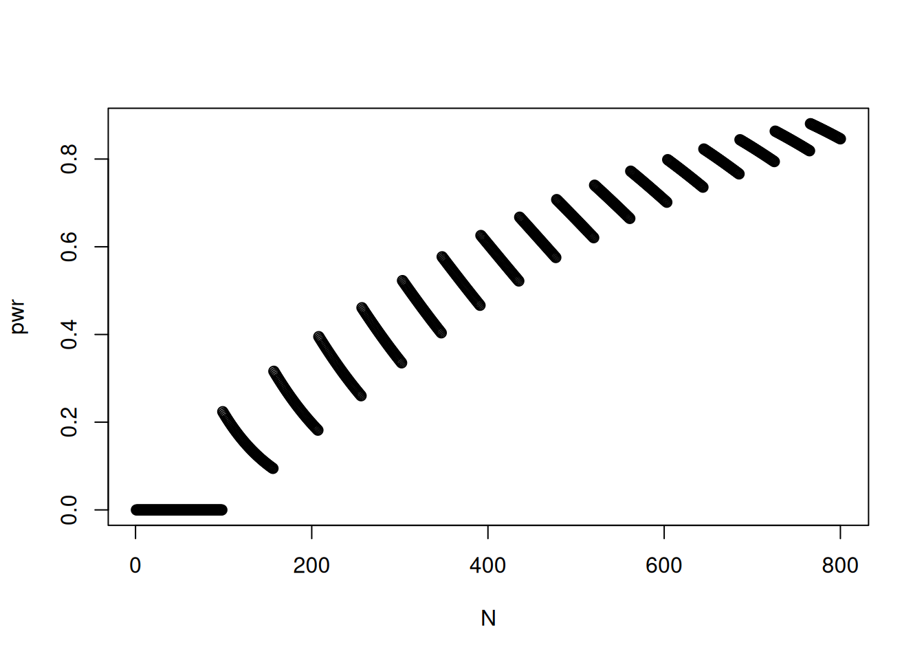
Or assessed for a sequence of \(n\) values (figure 15.1).

alpha <- 0.05
N <- 1:800 # Number of trials
pwr <- c() # Initiate vector for storage


for (n in N) {
  
  x <- 0:n
  
  nullProb <- pbinom(x, n, 0.03)
  
  xMax <- max(x[nullProb < alpha])
  pwr[n] <- pbinom(xMax, n, 0.015)
}

plot(N, pwr)

Figure 15.1: Power vs number of trials.

It is seen that indeed a very high number of samples needs to be collected in order to be fairly certain that the trial will statistically confirm that the number of nonconforming products has dropped.

Example 15.2 - Effect of caffeine on activity - power

The test in Example 10.1 reveal a p-value of p = 0.12 (see test below), which is not to be considered as strong support/evidence of a difference between the two groups. However, we do believe that there should be a difference between whether a mice is given water or red bull on their level of activity, and hence speculates that the study design is too small to be able to show a statistical significant difference between the two groups.

t.test(x_subset[x_subset$Caffeine == "Water", "RPM7"],
       x_subset[x_subset$Caffeine == "Red Bull", "RPM7"],
       var.equal = T)

    Two Sample t-test

data:  x_subset[x_subset$Caffeine == "Water", "RPM7"] and x_subset[x_subset$Caffeine == "Red Bull", "RPM7"]
t = -1.615, df = 18, p-value = 0.1237
alternative hypothesis: true difference in means is not equal to 0
95 percent confidence interval:
 -3.5208153  0.4604011
sample estimates:
mean of x mean of y 
 8.649382 10.179589 

The null hypothesis assumes equal means between the two groups. However, if we believe that this is not true. I.e. that there is a difference of say 2 points, then given a sample size of \(n \ ( = n1 + n2)\) what is the chance that the study turns out to give data that accepts (or rejects) the null hypothesis of no difference?

To answer this, we simulate a bunch of trials and check how many times \(H0\) is accepted:

m1 <- 8 # Mean of group 1
m2 <- 10 # Mean of group 2

s <- 2.1 # Standard deviation in both groups

n1 <- n2 <- 10 # Number of observations in each group

set.seed(2000) # Set seed for reproducibility of simulation

x1 <- rnorm(n1, m1, s) # Simulated normal distributed data for group 1
x2 <- rnorm(n2, m2, s) # Simulated normal distributed data for group 2

t.test(x1, x2, var.equal = T)$p.value # p-value from t-test

[1] 0.08542594

In this first trial \(p = 0.085\) and \(H0\) is hence accepted.

Now, let us simulate this 1000 times to see how often the null-hypothesis is accepted.

k <- 1000 # Number of simulations
p_values <- numeric(k) # Initialize vector for storage of values


for (i in 1:k) {
  
  x1 <- rnorm(n1, m1, s) # Simulated normal distributed data for group 1
  x2 <- rnorm(n2, m2, s) # Simulated normal distributed data for group 2
  
  p_values[i] <- t.test(x1, x2, var.equal = T)$p.value # p-value from t-test
  
}

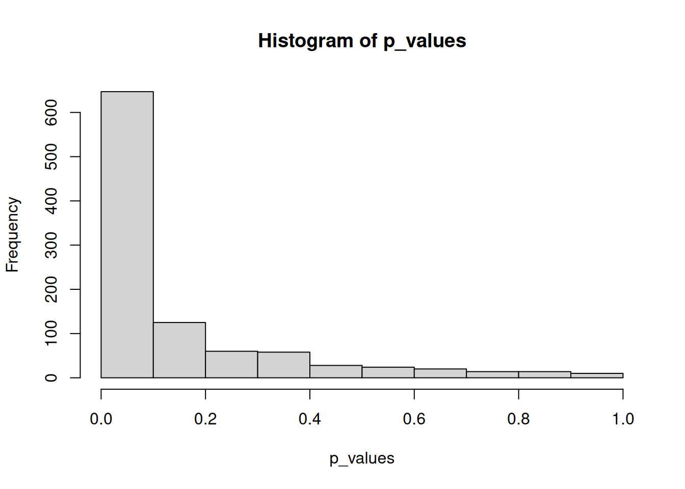
We now have a vector of p-values from 1000 simulations.

hist(p_values)

We can calculate how big a fraction of these simulated p-values that are under 0.05. That is, how many times the null-hypothesis was rejected.

sum(p_values < 0.05) / k

[1] 0.501

For the \(1000\) repeated trials half of them (\(501\) out of \(1000\)) accepts \(H0\) even thoug WE KNOW that the two groups are different (as they were simulated to be).

As such this is unacceptable, and we need to increase the power of our study.

There are several ways to increase the power:

• The two groups can be selected to be even more different (increse the effect size).
• The spread could be lowered.
• The number of observations (\(n1\) and \(n2\)) could be increased.

The function in R power.t.test() calculates the power as a function of these different settings.

power.t.test(delta = m2 - m1, sd = s, power = 0.8)

     Two-sample t test power calculation 

              n = 18.31862
          delta = 2
             sd = 2.1
      sig.level = 0.05
          power = 0.8
    alternative = two.sided

NOTE: n is number in *each* group

So, in order to achieve a power of \(0.8\) with the current population settings (mean and std) at least \(18.3\) samples (\(n1 = n2 = 18.3\)) should be included in each group of the study.

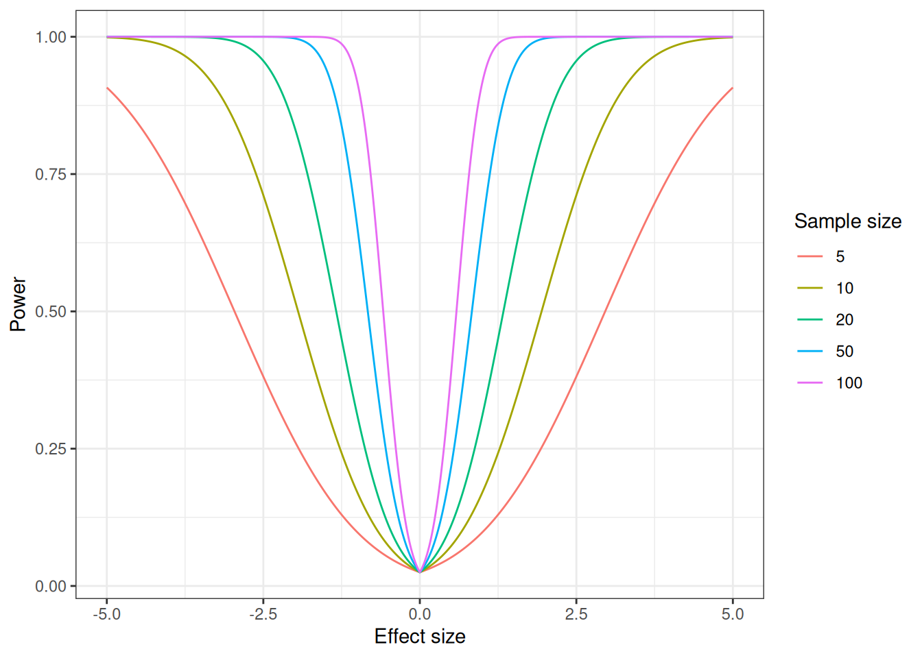
A more generic overview can also be achieved, where the power is calculated based on effect size (x-axis) and number of samples.

effect_sizes <- seq(-5, 5, by = 0.01) # Vector of effect sizes (delta)
sample_sizes <- c(5, 10, 20, 50, 100) # Vector of sample sizes (n)

pwr_df <- data.frame() # Empty data frame for storage

for (n in sample_sizes) { # Calculate for each sample size

  pwr <- power.t.test(delta = effect_sizes, sd = s, n = n)$power
    
  # Add data row by row
  pwr_df <- rbind(pwr_df, 
                  data.frame(delta = effect_sizes, N = n, power = pwr))
  
}

# Plot data
ggplot(pwr_df, aes(delta, power, color = factor(N))) +
  geom_line() +
  labs(
    x = "Effect size",
    y = "Power",
    color = "Sample size"
  ) +
  theme_bw()

15.3 Videos

15.3.1 Playing with Power: P-Values Pt 3 - CrashCourse

15.3.2 Power Analysis, Clearly Explained - StatQuest

15.3.3 Visualizing a Power Calculation - NCSS Statistical Software

15.3.4 Calculating Power in R - Ed Boone

15.4 Exercises

Exercise 15.1

Exercise 15.1 - Comparison of senses

A study wants to compare two types of trout samples, being meat stored under different conditions. The instrument used is a sensorical panel of 23 judges using either their visual sense, smelling sense or tasting sense. At each trial, each judges is presented with three pieces of meat - two similar and one odd. The task for the judge is to identify the odd sample using one of the senses. Data from such an experiment is presented in table 15.1.

Table 15.1: Data from a sensory study using 23 judges.

	Correct	Not correct
Smell	14	9
Taste	16	7
Visual appearance	22	1

Tasks

1. For now, stick to the sense Taste. State a statistical model for the outcome of each trial.
2. Formulate a null hypothesis based on the model, and test how different the observed results are compared to this hypothesis.

Based on the previous result, it seems like the different meat pieces is identifiable based on tasting. Now the questions is whether the two other senses performs similar in identification of the odd sample? (Hint: In this exercise you should use the method sketched in Method 7.19 and Method 7.21 in Brockhoff.)

Tasks

3. Give a frank ranking of the senses based on the observed data.
4. Formulate a model for each of the three senses.
5. State a null hypothesis in relation to the question of similarity between senses.
6. Compute by hand the expected values under this null hypothesis, \(\chi^2_{obs}\) and the degrees of freedom.
7. Use pchisq() to test the null hypothesis.
8. Test the hypothesis using a function in R (try to figure out which one that does the job in a single line) - compare the results with your own calculation.
9. Report the results in such a way, that differences between the three senses are communicated.
   • Hint: This can either be done by pairwise contrasts or confidence intervals for the central parameters.

Exercise 15.2

Exercise 15.2 - Our sensorical trial

In September 2015 the students in food science conducted two sensorical trials. A triangle test and a duo trio test. Both on apple juice for discrimination between normal juice and juice with added citric acid. In table 15.2 is listed the results from the 69 judges in the study.

Table 15.2: Results of the two sensorical trials.

	N	Correct
Duo-Trio	29	12
Triangle	40	20

Tasks

1. What is the chance probability for answering correct in the two tests?
2. Initially, inspect data to see how the frequencies of correct answers compare with the chance probability. Can you draw conclusions without doing any stats?
3. State two models for the data obtained from the Duo-trio test and from the triangle test.
4. State null- and alternative hypothesis for the relevant data.
5. Calculate the probability of observing the results (and what is more extreme compared to the null hypothesis) under the null-assumption.
6. In case of rejection of the null hypothesis, give a estimate (and confidence interval) for the parameter.
7. How big is the proportion of people who are actually able to taste differences based on this result?
   • Hint: you need to take into account the amount of people who gives correct answer by guessing.

Exercise 15.3

Exercise 15.3 - Power calculation - triangle test

A chocolate company have a product, which they want to improve the quality of. In order to do so, they change some of the raw material to a more expensive alternative. In order to test whether this change actually ”pays of” they set up an experiment - A triangle test. Among a set of consumers (\(n\)), each consumer is presented to three pieces of chocolate, two of type \(A\) and one of type \(B\), with the task of finding type \(B\). The recorded data from such an experiment may look like:

\[ 0,0,1,0,1,1,...0 \]

Tasks

1. Write up the statistical model underlying these data.
2. If it is not possible to identify type \(B\), what is the value of the parameter?

A trial based on responses from 20 consumers results in half (\(x = 10\)) correctly identified.

Tasks

3. What is the probability of observing such a results (or more extreme) under the null hypothesis of no differences between type \(A\) and type \(B\)?

The product manager is not satisfied with the results, after all half of the consumers were able to distinguish he says. You think 50% - Aaahhh that is not actually what the data says - some of them were random!, but you leave it there, as your boss is from CBS and basically without any technical insight!, so instead you assumme that this is indeed the case for the entire population (that the probability of selecting type \(B\) is \(p = 0.5\)).

Tasks

4. How many customers should you include in your trial in order to have a fair chance of achieving a significant result?
   • Hint i: Calculate for \(n = 20, 21, ...\) the least number of correct findings in order for the results to be significant under the null hypothesis. I.e. what is \(x\) in \(P(X ≥ x) < 0.05\) under \(p = p0\) (the guessing probability).
   • Hint ii: Calculate the probability of observing this (and more extreme) given the population probability of \(p = 0.5\).
5. Plot the combination of number of customers (\(n\)) and the probability of getting significant results, and device a new trial.

Exercise 15.4

Exercise 15.4 - Triangle or Duo-Trio?

There exist a bunch of sensorical discrimination test, which all have the same aim, but are different in setup. In this exercise we are going to deal with the power of Triangle test and Duo-Trio test.

Tasks

1. State the statistical model for the two test types.
2. State the chance probabilities, and formulate null- and alternative hypothesis, for both tests.
3. Now assume you conduct both trials \(n = 20\) times. What is the least number of correct answers needed to get significant discrimination between the products.
4. Assume that 50% of the people in the population are actually able to discriminate the samples. What is the expected frequency of correct answers under this assumption?
   • HINT: think of 100 persons.
5. Calculate the power for a Duo-trio and a Triangle test with \(n = 20\) assuming these populations probabilities.
6. Comment on why somebody still uses the Duo-trio test.

Exercise 15.5

Exercise 15.5 - Power calculation in T-test

Short version
You have been able to isolate a fiber from a novel source. With the increasing lifestyle related health problems, you think that your new fiber might actually* save the world*. You just need to prove it. In order to do so, you set up an experiment similar to the one described in “Fiber and Cholesterol”. I.e. a paired setup with baseline measurements, followed by an intervention period and end-of-trial measurements. You will have proven your case if the fiber supplemented to the diet is able to lower the cholesterol level. The question is: How many patients do you need in order to run such a trial?

Long version
You have been able to isolate a fiber from a novel source. With the increasing lifestyle related health problems, you think that your new fiber might actually* save the world*. You just need to prove it. In order to do so, you set up an experiment similar to the one described in “Fiber and Cholesterol”. I.e. a paired setup with baseline measurements, followed by an intervention period and end-of-trial measurements. You will have proven your case if the fiber supplemented to the diet is able to lower the cholesterol level. The question is: How many patients do you need in order to run such a trial?

Tasks

1. Based on your knowledge on fiber and health give some numbers for effect size, and standard deviation.
   • Hint: You might use the results from a previous similar study to get reliable numbers.
2. Write up the test statistics for this experiment.
3. Calculate the test statistics for varying number of included persons, with the parameters (effect size and standard deviation) fixed.
4. Use the function power.t.test() to calculate how many persons are needed for a trial with power of \(\beta = 0.80\) and a significance threshold of \(\alpha = 0.05\).