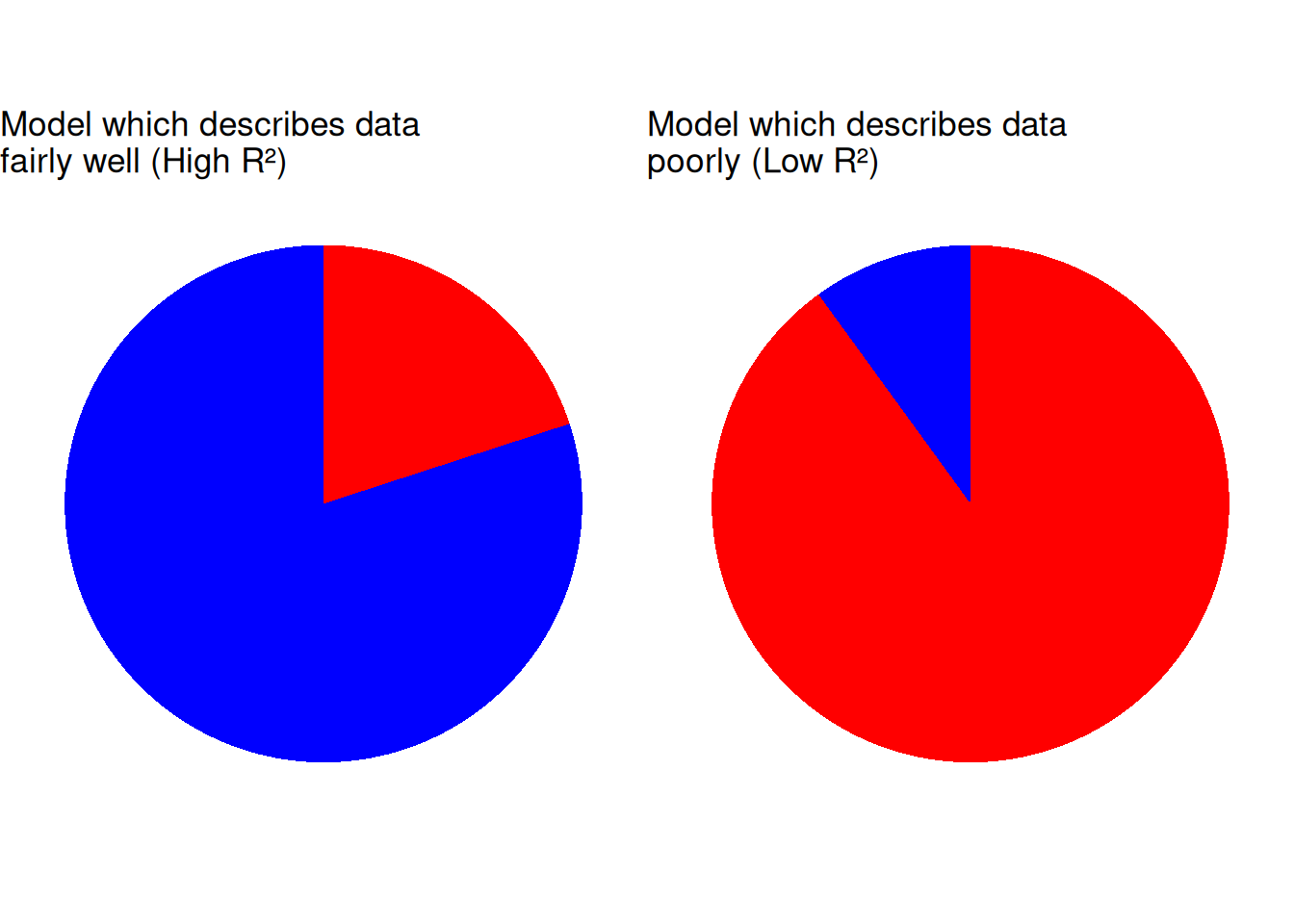
Explained variance refers to how well the estimated model describes the observed data. That is, how much of the variation is systematic and how much is residual. In the figure below are shown two examples.
Figure 21.1: Systematic variation (blue) and residual variation (red).
The explained variance is summarized in the so-called \(R^2 \in \left[ 0,1 \right]\) metric. Where a value close to \(1\) indicates high degree of explained variance, and a value close to \(0\) the contrary.
\(R^2\) is based on the sums of squares of the different model terms. Given the model:
\[
X = S + E
\]
Where \(X\) refers to the observed data, \(S\) the systematic parameterized part of the model and \(E\) the residuals, then:
\[
SS(X) = SS(S) + SS(E)
\]
I.e. the sums of squares are additive. From this the \(R^2\) value is defined as:
In both ANOVA and linear regression these \(SS()\) values are readily available from the analysis table, where \(SS(X) = SS_{tot}\) and \(SS(E) = SS_e\). Further, it is possible to calculate the \(R^2\) for the entire model, but also for individual factors in twoway ANOVA and regression with multiple descriptors, simply by using the individual \(SS()\) contributions.
21.2.1 Model estimates (\(\hat{y}\)) and \(R^2\)
In linear regression the model is stated as:
\[
\begin{gather}
y_{i} = \alpha + \beta \cdot x_i + e_i \\
where \ e_{i}\sim \mathcal{N}(0,\sigma^2) \ and \ independent \\
for \ i=1,...,n
\end{gather}
\]
The predicted values for \(y\) (referred to as \(\hat{y}\)) can be expressed as:
where the estimates of the slope and the intercept is used for calculating \(y\) based on \(x\).
The \(R^2\) value for such a model can also be seen as:
\[
R^2 = r_{\hat{y},y}^2
\]
That is, taking the squared value of the correlation coefficient between the observed response and the predicted response yields the explained variance by the model.
This concept is valid for for a range of models including ANOVA, PCA and linear regression.
21.2.2 Correlation coefficient and \(R^2\)
In bi-variate correlation analysis, the correlation coefficient is directly related to \(R^2\), as: I
The implication of this, is that the direction is lost (\(R^2 = 0.3^2 = (-0.3)^2\)), but the strength of the relation is not.
21.2.3\(R^2\) for PCA
In a PCA model, it is possible to talk about \(R^2\) values for the entire model or for the individual components. It is so, by definition, that the contribution from the individual components is decreasing, that is:
In PCA, by increasing the number of components you will eventually reach explained variance of \(1\). This is due to the parameters of this model is solely based on the response variables, so there is no set of independent variables, as there is in ANOVA and linear regression. This has the implication, that comparing \(R^2\) values between e.g. an ANOVA model and a PCA model is not at all straight forward.
21.3 Videos
What does r squared tell us? What does it all mean - MrNystrom
This exercise deals with explained variance and its relation to the residual deviation. This exercise uses the dietary intervention on mice and the effect on biomarkers related to fat metabolism.
Tasks
First, we are going to deal with insulin and cholesterol. Make three analyses:
Regress cholesterol on insulin.
Regress insulin on cholesterol.
Make a correlation analysis between the two.
Make a drawing (not exact, just some dots) of cholesterol versus insulin and indicate a regression line, and the the residuals for the first two models in Q1.
For each model, calculate \(R^2\).
Hint: You can use the \(SS\) measures of an aov() model, or use summary() of a lm() model directly.
Comment on what you observe.
Exercise 21.2
Exercise 21.2 - R-squared and outliers
This exercise should show how extreme outliers can influence the \(R^2\) measure by making it unrealistically high.
Tasks
Simulate two sets of vector \(x\) and \(y\), each of \(n=15\) points which are not related. (use rnorm() in R for doing so).
Scatter plot \(x\) and \(y\) and add the best regression line. (code hint: + stat_smooth(method = "lm"))
Calculate the correlation coefficient (\(r\)) and the \(R^2\) value.
Do the stats (\(r\) and \(R^2\)) and the plot tells the same story?
Now add an extreme point to both \(x\) and \(y\) (x <- c(x,extremenumber)).
Repeat plotting and stat calculation (\(r\) and \(R^2\)).
What happened?
Important
Take home message: \(R^2\) alone without visual inspection can be misleading.
Exercise 21.3
Exercise 21.3 - R-squared and transformations
This exercise should show how transformation influences the \(R^2\) measure. The exercise is using the wine dataset.
Tasks
Import data, and make a plot of the response variable Ethyl.pyruvate inferring country membership.
Make a oneway ANOVA model for this response variable, and check (or calculate) the \(R^2\) value.
Make a transformation of the response variable, and repeat plotting, modeling and \(R^2\) calculation.
Compare the \(R^2\) for the raw response and transformed response, and figure out (based on the plots) which samples that are causing the difference.
Make a check of model assumptions for both models, and try to fix the issues by outlier removal.
Hint: a simple way to remove samples and update models can be seen below.
ic <- wine$Ethyl.pyruvate < ...m <-lm(data = wine[ic, ], ...)
Exercise 21.4
Exercise 21.4 - Explained variance and PCA
This exercise deals with explained variance in relation to PCA. This exercise uses the dietary intervention on mice and the effect on biomarkers related to fat metabolism.
Tasks
Initially extract and scale the biomarkers in the dataset (use X <- scale() for this purpose).
Calculate the total sums of squares for these data? (sum(X^2))
Calculate a PCA model on these preprocessed data, and plot it using ggbiplot().
Calculate the residuals after the first component. This is done by calculating the predicted values and subtracting those from the data (see code below).
# "pca" refers to a PCA model built by "prcomp()"Xhat <- pca$x[ , 1] %o% mm$rotation[ , 1]E <- X - Xhat
Tasks
Calculate the residual sums of squares after removing the first component.
Calculate the \(R^2\) for the first component.
Try to calculate the \(R^2\) value from the correlation between \(\mathbf{X}\) and \(\hat{\mathbf{X}}\): CODE HERE
Try to modify the code in Q4 to be able to calculate for component \(2\), \(3\),…
Eventually you can match your results with the ones produced by ggbiplot().
Source Code
# Explained variance```{r}#| label: exp-var-setup#| echo: false#| message: false#| warning: falselibrary(ggplot2)library(gridExtra)```::: {.callout-tip}## Learning objectivesThe learning objectives for this theme are to:* Understand the general notion of explained variance and its relation to least squares.:::## Reading material* [Explained variance - in short](#sec-explained-var-intro)* Videos on R-squared: * [What does r squared tell us? What does it all mean](#sec-r2-mrnystrom) * [R-squared, Clearly Explained](#sec-r2-statquest)## Explained variance - in short {#sec-explained-var-intro}Explained variance refers to how well the estimated model describes the observed data. That is, how much of the variation is systematic and how much is residual. In the figure below are shown two examples.```{r}#| label: fig-r2-pies#| fig-cap: Systematic variation (blue) and residual variation (red). #| echo: falsegood_fit <-data.frame(category =c("Explained", "Unexplained"),value =c(0.8, 0.2) )poor_fit <-data.frame(category =c("Explained", "Unexplained"),value =c(0.1, 0.9))p1 <-ggplot(good_fit, aes(x ="", y = value, fill = category)) +geom_bar(stat ="identity", width =1) +coord_polar("y", start =0) +scale_fill_manual(values =c("blue", "red")) +theme_void() +theme(legend.position ="none") +ggtitle("Model which describes data\nfairly well (High R²)")p2 <-ggplot(poor_fit, aes(x ="", y = value, fill = category)) +geom_bar(stat ="identity", width =1) +coord_polar("y", start =0) +scale_fill_manual(values =c("blue", "red")) +theme_void() +theme(legend.position ="none") +ggtitle("Model which describes data\npoorly (Low R²)")grid.arrange(p1, p2, ncol =2)```The explained variance is summarized in the so-called $R^2 \in \left[ 0,1 \right]$ metric. Where a value close to $1$ indicates high degree of explained variance, and a value close to $0$ the contrary.$R^2$ is based on the sums of squares of the different model terms. Given the model:$$X = S + E$$Where $X$ refers to the observed data, $S$ the systematic parameterized part of the model and $E$ the residuals, then:$$SS(X) = SS(S) + SS(E)$$I.e. the sums of squares are additive. From this the $R^2$ value is defined as:$$R^2 = \frac{SS(S)}{SS(X)} = \frac{SS(X) - SS(E)}{SS(X)} = 1 - \frac{SS(E)}{SS(X)}$$In both ANOVA and linear regression these $SS()$ values are readily available from the analysis table, where $SS(X) = SS_{tot}$ and $SS(E) = SS_e$. Further, it is possible to calculate the $R^2$ for the entire model, but also for individual factors in twoway ANOVA and regression with multiple descriptors, simply by using the individual $SS()$ contributions.### Model estimates ($\hat{y}$) and $R^2$In linear regression the model is stated as:$$\begin{gather}y_{i} = \alpha + \beta \cdot x_i + e_i \\where \ e_{i}\sim \mathcal{N}(0,\sigma^2) \ and \ independent \\for \ i=1,...,n\end{gather}$$The predicted values for $y$ (referred to as $\hat{y}$) can be expressed as:$$\hat{y}_{i} = \hat{\alpha} + \hat{\beta} \cdot x_i$$where the estimates of the slope and the intercept is used for calculating $y$ based on $x$.The $R^2$ value for such a model can also be seen as:$$R^2 = r_{\hat{y},y}^2$$That is, taking the squared value of the correlation coefficient between the observed response and the predicted response yields the explained variance by the model.This concept is valid for for a range of models including ANOVA, PCA and linear regression.### Correlation coefficient and $R^2$In bi-variate correlation analysis, the correlation coefficient is directly related to $R^2$, as:IThe implication of this, is that the *direction* is lost ($R^2 = 0.3^2 = (-0.3)^2$), but the *strength* of the relation is not.### $R^2$ for PCAIn a PCA model, it is possible to talk about $R^2$ values for the entire model or for the individual components. It is so, by definition, that the contribution from the individual components is decreasing, that is:$$R_{PC1}^2 \geq R_{PC2}^2 \geq \ldots \geq R_{PCk}^2$$Further, from a $k$ component model follows that total explained variance is:$$R_{PC1-PCk}^2 = R_{PC1}^2 + R_{PC2}^2 + \ldots + R_{PCk}^2 = \sum_{i=1}^k{R_{PCi}^2}$$#### PCA vs Regression/ANOVAIn PCA, by increasing the number of components you will eventually reach explained variance of $1$. This is due to the parameters of this model is solely based on the response variables, so there is no set of independent variables, as there is in ANOVA and linear regression. This has the implication, that comparing $R^2$ values between e.g. an ANOVA model and a PCA model is not at all straight forward.## Videos#### What does r squared tell us? What does it all mean - *MrNystrom* {#sec-r2-mrnystrom}{{< video https://www.youtube.com/watch?v=IMjrEeeDB-Y >}}#### R-squared, Clearly Explained - *StatQuest* {#sec-r2-statquest}{{< video https://www.youtube.com/watch?v=bMccdk8EdGo >}}## Exercises::: {#ex-explained-variance}<!-- Cross-ref anchor -->:::::: {.callout-exercise}### Explained variance (R-squared) - regression n' correlationThis exercise deals with explained variance and its relation to the residual deviation. This exercise uses the dietary intervention on mice and the effect on biomarkers related to fat metabolism.::: {.callout-task}1. First, we are going to deal with insulin and cholesterol. Make three analyses: a. Regress cholesterol on insulin. b. Regress insulin on cholesterol. c. Make a correlation analysis between the two.2. Make a drawing (not exact, just some dots) of cholesterol versus insulin and indicate a regression line, and the the residuals for the first two models in Q1.3. For each model, calculate $R^2$. * Hint: You can use the $SS$ measures of an `aov()` model, or use `summary()` of a `lm()` model directly.4. Comment on what you observe.::::::<!-- End exercise callout -->::: {#ex-r2-and-outliers}<!-- Cross-ref anchor -->:::::: {.callout-exercise}### R-squared and outliersThis exercise should show how extreme outliers can influence the $R^2$ measure by making it unrealistically high.::: {.callout-task}1. Simulate two sets of vector $x$ and $y$, each of $n=15$ points which are not related. (use `rnorm()` in R for doing so).2. Scatter plot $x$ and $y$ and add the best regression line. (code hint: `+ stat_smooth(method = "lm")`)3. Calculate the correlation coefficient ($r$) and the $R^2$ value.4. Do the stats ($r$ and $R^2$) and the plot tells the same story?5. Now add an extreme point to both $x$ and $y$ (`x <- c(x,extremenumber)`).6. Repeat plotting and stat calculation ($r$ and $R^2$).7. What happened?:::::: {.callout-important}Take home message: $R^2$ alone without visual inspection can be misleading.::::::<!-- End exercise callout -->::: {#ex-r2-and-transformations}<!-- Cross-ref anchor -->:::::: {.callout-exercise}### R-squared and transformationsThis exercise should show how transformation influences the $R^2$ measure. The exercise is using the wine dataset.::: {.callout-task}1. Import data, and make a plot of the response variable `Ethyl.pyruvate` inferring country membership.2. Make a oneway ANOVA model for this response variable, and check (or calculate) the $R^2$ value.3. Make a transformation of the response variable, and repeat plotting, modeling and $R^2$ calculation.4. Compare the $R^2$ for the raw response and transformed response, and figure out (based on the plots) which samples that are causing the difference.5. Make a check of model assumptions for both models, and try to fix the issues by outlier removal. * Hint: a simple way to remove samples and update models can be seen below.:::```{r}#| eval: falseic <- wine$Ethyl.pyruvate < ...m <-lm(data = wine[ic, ], ...)```:::<!-- End exercise callout -->::: {#ex-exp-var-and-pca}<!-- Cross-ref anchor -->:::::: {.callout-exercise}### Explained variance and PCAThis exercise deals with explained variance in relation to PCA. This exercise uses the dietary intervention on mice and the effect on biomarkers related to fat metabolism.::: {.callout-task}1. Initially extract and scale the biomarkers in the dataset (use `X <- scale()` for this purpose).2. Calculate the total sums of squares for these data? (`sum(X^2)`)3. Calculate a PCA model on these preprocessed data, and plot it using `ggbiplot()`.4. Calculate the residuals after the first component. This is done by calculating the predicted values and subtracting those from the data (see code below).:::```{r}#| eval: false# "pca" refers to a PCA model built by "prcomp()"Xhat <- pca$x[ , 1] %o% mm$rotation[ , 1]E <- X - Xhat```::: {.callout-task}5. Calculate the residual sums of squares after removing the first component.6. Calculate the $R^2$ for the first component.7. Try to calculate the $R^2$ value from the correlation between $\mathbf{X}$ and $\hat{\mathbf{X}}$: CODE HERE8. Try to modify the code in Q4 to be able to calculate for component $2$, $3$,...:::Eventually you can match your results with the ones produced by `ggbiplot()`.:::<!-- End exercise callout -->